Faster numerical inverse Laplace transform in mpmath

Recently, I was numerically inverting computationally expensive Laplace transforms. I was looking for methods requiring as few terms as possible while showing numerical robustness. My first approach was to look at the implementation in mpmath and experiment with basic examples. As detailed in the documentation, the default method dehoog was the most reliable at the expense of significant CPU times as the desired precision increases. Since I was not fully satisfied with the performance I decided to develop an alternative method.

Algorithm

This alternative method uses the Bromwich contour inversion integral given by: $$ f(t) = \mathcal{L}^{-1}\{\mathcal{L}\{f\}(s)\}(t) = \frac{1}{2\pi i}\int_{a - i\infty}^{a + i\infty} e^{st} \mathcal{L}\{f\}(s) \mathop{ds}\\ = \frac{2 e^{at}}{\pi}\int_0^{\infty} \Re\left(\mathcal{L}\{f\}(a + iu) \right) \cos(ut) \mathop{du}. $$ The contour integral can be replaced by a nearly alternating series obtained after application of the trapezoidal rule to with step \(h = \frac{\pi}{2 t}\) and abscissa \(a= \frac{\gamma}{2 t}\), $$f_h(t) = \frac{e^{\gamma / 2}}{t} \left[\frac{1}{2}\Re\left(\hat{f}\left(\frac{\gamma}{2t}\right) \right) - \sum_{k=0}^{\infty}(-1)^k\Re\left(\bar{f}\left(\frac{\gamma + 2(k+1) \pi i}{2t}\right)\right)\right],$$ where we use \(\bar{f}(s) = \mathcal{L}\{f\}(s)\}\) to simplify notation. A widely used value for \(\gamma\), suggested in (Abate, Whitt, 1995), is \(d \log(10)\), where \(d\) is the number of digits. A more numerically stable formula for \(\gamma\) in terms of \(t\) is developed in (Glasserman, Ruiz-Mata, 2006): $$\gamma = \frac{2}{3} (d \log(10) + \log(2 t)).$$ In my experiments, the latter value improves the approximation error, especially as \(t\) grows; therefore, this is the selected formula for the implementation.

The above series suffers the same slow convergence issue than the Fourier series used by dehoog. To accelerate convergence, we can use methods such as Euler-Van Wijngaarden with convergence \(\mathcal{O}(2^{-M})\) or the Padé-approximation in (de Hoog et al, 1982). Alternatively, we could use the linear acceleration method in (Cohen et al, 2000) with convergence \(\mathcal{O}(5.828^{-M})\). This linear acceleration is convenient for arbitrary-precision since the coefficients can be computed without additional storage, and requires \(M = \lceil 1.31 d \rceil\) terms in the approximation. Given an alternating series \(S = \sum_{k=0}^{\infty} (-1)^k a_k\), the relative error of the approximation, \(S_M\) is: $$\frac{|S - S_M|}{|S|} \approx \frac{2}{(3+\sqrt{8})^M}.$$ Finally, taking \(a_k = \Re\left(\bar{f} \left(\frac{\gamma + 2(k+1) \pi i}{2t}\right)\right)\), we get $$f(t, M) = \frac{e^{\gamma / 2}}{t} \left[\frac{1}{2} \Re\left(\bar{f}\left(\frac{\gamma}{2t}\right) \right) - \sum_{k=0}^{M-1}\frac{c_{M,k}}{d_M}\Re\left(\bar{f} \left(\frac{\gamma + 2(k+1) \pi i}{2t}\right)\right)\right],$$ where $$c_{M,k} = (-1)^k \left(d_M - \sum_{m=0}^k \frac{M}{M+m} \binom{M+m}{2m}\right), \quad d_M = \frac{(3+\sqrt{8})^M + (3-\sqrt{8})^M}{2}.$$ Note that the linear acceleration method works even though the series is not exactly alternating.

Numerical experiments

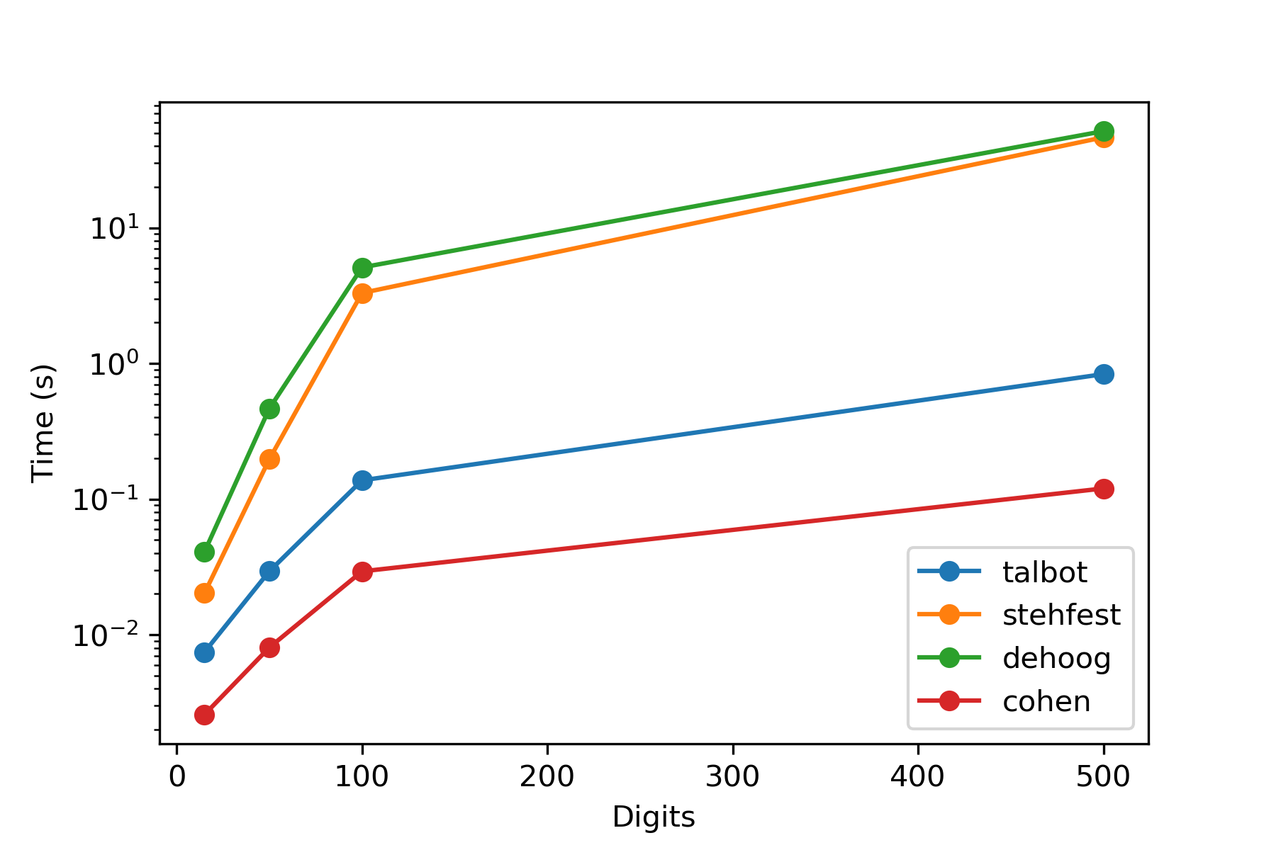
Here we see how the presented method compares to the three methods currently implemented in mpmath. I have named this method cohen as a reference to the linear acceleration method used. In all cases, the four methods are evaluated with (15, 50, 100, 500) digits of precision.

Case 1: $$\bar{f}(p) = \frac{1}{(p+1)^2}, \qquad f(t) = t e^{-t}$$ All four methods return the correct value, and only the stehfest method shows some loss of precision (between 18 and 22 digits) at 500 digits. In terms of timing, the cohen shows superior performance, more than two orders of magnitude faster than the default method dehoog.

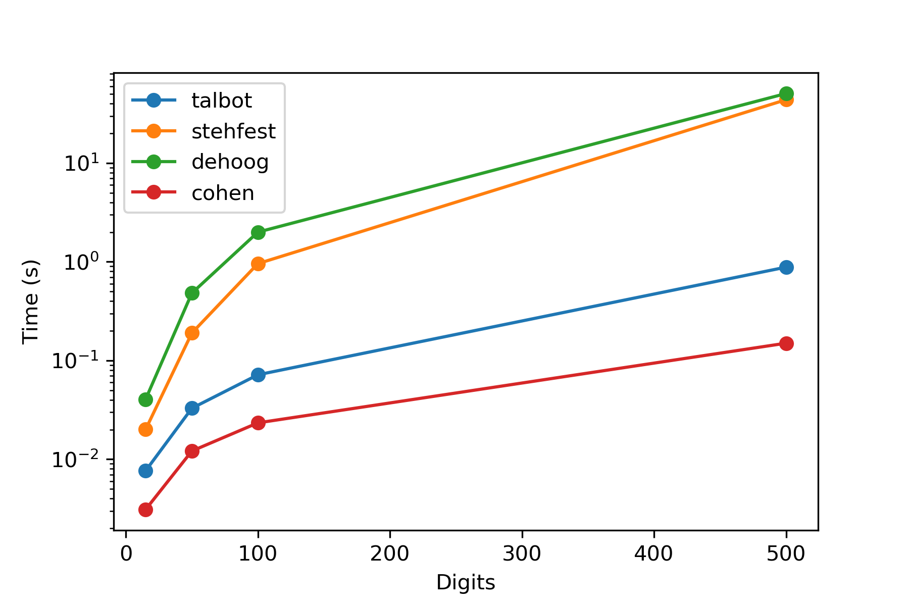
Case 2: $$\bar{f}(p) = \frac{1}{p^2+1}, \qquad f(t) = J_0(t)$$ In this case, the talbot method barely achieves more than a few correct digits independently of the desired precision. The method stehfest shows loss of precision at 15, 50 and 500 digits, evidencing the behaviour described in the documentation. Regarding CPU times, the conclusion follows case 1.

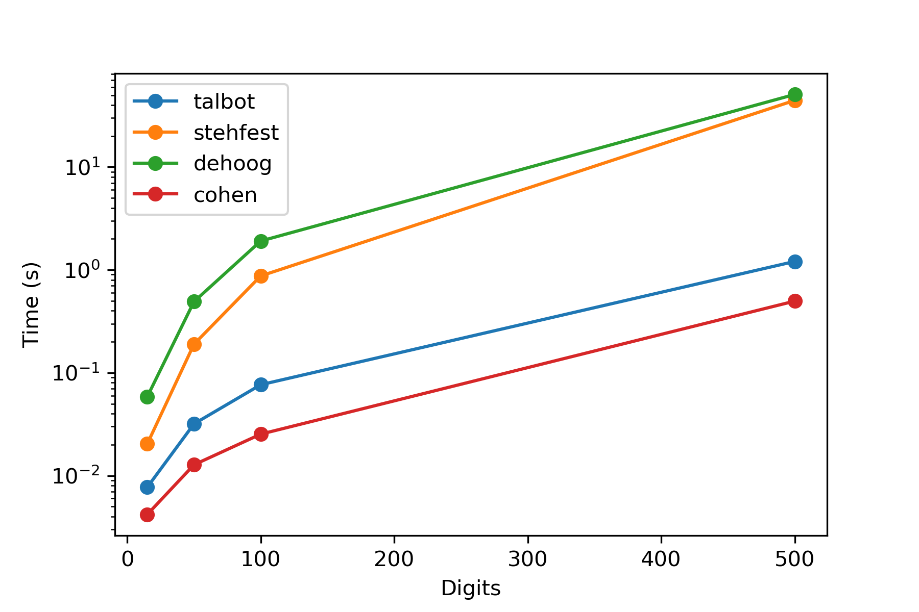
Case 3: $$\bar{f}(p) = \frac{\log(p)}{p}, \qquad f(t) = -\gamma - \log(t),$$ where \(\gamma \) is the Euler–Mascheroni constant. For this case, all four methods achieve the desired precision. The difference in terms of performance does not vary.

Implementation

The implementation can be found in my GitHub branch. It is worth noting that the invertlaplace method could be enhanced by parallelizing the evaluation of \(\bar{f}(p_k), \, k = 1,\ldots, M\) using multiprocessing.

References

• J. Abate and W. Whitt (1995). Numerical inversion of the Laplace transforms of probability distributions. ORSA Journal on Computing, 7(1):36-43
• H. Cohen, F. Rodriguez Villegas, and D. Zagier (2000). Convergence acceleration of alternating series. Experimental Mathematics, 9(1):3-12
• P. Glasserman and J. Ruiz-Mata (2006). Computing the credit loss distribution in the Gaussian copula model: a comparison of methods. Journal of Credit Risk, 2(4):33-66
• F. R. de Hoog, J. H. Knight, and A. N. Stokes (1982). An improved method for numerical inversion of Laplace transforms SIAM Journal on Scientific and Statistical Computing, 3(3):357-366.