Tutorial: optimal binning with binary target¶

Basic¶

To get us started, let’s load a well-known dataset from the UCI repository and transform the data into a pandas.DataFrame.

[1]:

import numpy as np
import pandas as pd
from sklearn.datasets import load_breast_cancer

[2]:

data = load_breast_cancer()
df = pd.DataFrame(data.data, columns=data.feature_names)

We choose a variable to discretize and the binary target.

[3]:

variable = "mean radius"
x = df[variable].values
y = data.target

Import and instantiate an OptimalBinning object class. We pass the variable name, its data type, and a solver, in this case, we choose the constraint programming solver.

[4]:

from optbinning import OptimalBinning

[5]:

optb = OptimalBinning(name=variable, dtype="numerical", solver="cp")

We fit the optimal binning object with arrays x and y.

[6]:

optb.fit(x, y)

[6]:

OptimalBinning(name='mean radius')

You can check if an optimal solution has been found via the status attribute:

[7]:

optb.status

[7]:

'OPTIMAL'

You can also retrieve the optimal split points via the splits attribute:

[8]:

optb.splits

[8]:

array([11.42500019, 12.32999992, 13.09499979, 13.70499992, 15.04500008,
       16.92500019])

The binning table¶

The optimal binning algorithms return a binning table; a binning table displays the binned data and several metrics for each bin. Class OptimalBinning returns an object BinningTable via the binning_table attribute.

[9]:

binning_table = optb.binning_table

[10]:

type(binning_table)

[10]:

optbinning.binning.binning_statistics.BinningTable

The binning_table is instantiated, but not built. Therefore, the first step is to call the method build, which returns a pandas.DataFrame.

[11]:

binning_table.build()

[11]:

	Bin	Count	Count (%)	Non-event	Event	Event rate	WoE	IV	JS
0	(-inf, 11.43)	118	0.207381	3	115	0.974576	-3.125170	0.962483	0.087205
1	[11.43, 12.33)	79	0.138840	3	76	0.962025	-2.710972	0.538763	0.052198
2	[12.33, 13.09)	68	0.119508	7	61	0.897059	-1.643814	0.226599	0.025513
3	[13.09, 13.70)	49	0.086116	10	39	0.795918	-0.839827	0.052131	0.006331
4	[13.70, 15.05)	83	0.145870	28	55	0.662651	-0.153979	0.003385	0.000423
5	[15.05, 16.93)	54	0.094903	44	10	0.185185	2.002754	0.359566	0.038678
6	[16.93, inf)	118	0.207381	117	1	0.008475	5.283323	2.900997	0.183436
7	Special	0	0.000000	0	0	0.000000	0.000000	0.000000	0.000000
8	Missing	0	0.000000	0	0	0.000000	0.000000	0.000000	0.000000
Totals		569	1.000000	212	357	0.627417		5.043925	0.393784

Let’s describe the columns of this binning table:

Bin: the intervals delimited by the optimal split points.
Count: the number of records for each bin.
Count (%): the percentage of records for each bin.
Non-event: the number of non-event records \((y = 0)\) for each bin.
Event: the number of event records \((y = 1)\) for each bin.
Event rate: the percentage of event records for each bin.
WoE: the Weight-of-Evidence for each bin.
IV: the Information Value (also known as Jeffrey’s divergence) for each bin.
JS: the Jensen-Shannon divergence for each bin.

The last row shows the total number of records, non-event records, event records, and IV and JS.

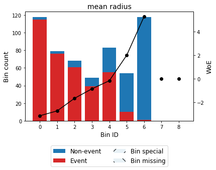
You can use the method plot to visualize the histogram and WoE or event rate curve. Note that the Bin ID corresponds to the binning table index.

[12]:

binning_table.plot(metric="woe")

../_images/tutorials_tutorial_binary_24_0.png

[13]:

binning_table.plot(metric="event_rate")

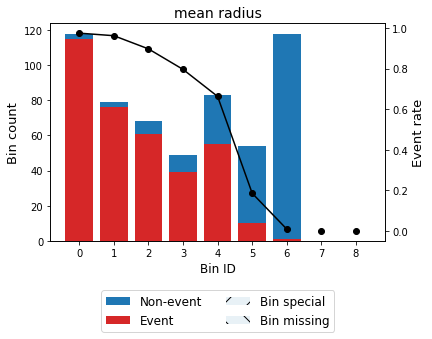
../_images/tutorials_tutorial_binary_25_0.png

Note that WoE is inversely related to the event rate, i.e., a monotonically ascending event rate ensures a monotonically descending WoE and vice-versa. We will see more monotonic trend options in the advanced tutorial.

Event rate / WoE transformation¶

Now that we have checked the binned data, we can transform our original data into WoE or event rate values. You can check the correctness of the transformation using pandas value_counts method, for instance.

[14]:

x_transform_woe = optb.transform(x, metric="woe")

[15]:

pd.Series(x_transform_woe).value_counts()

[15]:

-3.125170    118
 5.283323    118
-0.153979     83
-2.710972     79
-1.643814     68
 2.002754     54
-0.839827     49
dtype: int64

[16]:

x_transform_event_rate = optb.transform(x, metric="event_rate")

[17]:

pd.Series(x_transform_event_rate).value_counts()

[17]:

0.974576    118
0.008475    118
0.662651     83
0.962025     79
0.897059     68
0.185185     54
0.795918     49
dtype: int64

[18]:

x_transform_indices = optb.transform(x, metric="indices")

[19]:

pd.Series(x_transform_indices).value_counts()

[19]:

0    118
6    118
4     83
1     79
2     68
5     54
3     49
dtype: int64

[20]:

x_transform_bins = optb.transform(x, metric="bins")

[21]:

pd.Series(x_transform_bins).value_counts()

[21]:

(-inf, 11.43)     118
[16.93, inf)      118
[13.70, 15.05)     83
[11.43, 12.33)     79
[12.33, 13.09)     68
[15.05, 16.93)     54
[13.09, 13.70)     49
dtype: int64

Categorical variable¶

Let’s load the application_train.csv file from the Kaggle’s competition https://www.kaggle.com/c/home-credit-default-risk/data.

[22]:

df_cat = pd.read_csv("data/kaggle/HomeCreditDefaultRisk/application_train.csv",
                     engine='c')

[23]:

variable_cat = "NAME_INCOME_TYPE"
x_cat = df_cat[variable_cat].values
y_cat = df_cat.TARGET.values

[24]:

df_cat[variable_cat].value_counts()

[24]:

Working                 158774
Commercial associate     71617
Pensioner                55362
State servant            21703
Unemployed                  22
Student                     18
Businessman                 10
Maternity leave              5
Name: NAME_INCOME_TYPE, dtype: int64

We instantiate an OptimalBinning object class with the variable name, its data type (categorical) and a solver, in this case, we choose the mixed-integer programming solver. Also, for this particular example, we set a cat_cutoff=0.1 to create bin others with categories in which the percentage of occurrences is below 10%. This will merge categories State servant, Unemployed, Student, Businessman and Maternity leave.

[25]:

optb = OptimalBinning(name=variable_cat, dtype="categorical", solver="mip",
                      cat_cutoff=0.1)

[26]:

optb.fit(x_cat, y_cat)

[26]:

OptimalBinning(cat_cutoff=0.1, dtype='categorical', name='NAME_INCOME_TYPE',
               solver='mip')

[27]:

optb.status

[27]:

'OPTIMAL'

The optimal split points are the list of classes belonging to each bin.

[28]:

optb.splits

[28]:

[array(['Pensioner'], dtype=object),
 array(['Commercial associate'], dtype=object),
 array(['Working'], dtype=object),
 array(['State servant', 'Unemployed', 'Student', 'Businessman',
        'Maternity leave'], dtype=object)]

[29]:

binning_table = optb.binning_table
binning_table.build()

[29]:

	Bin	Count	Count (%)	Non-event	Event	Event rate	WoE	IV	JS
0	[Pensioner]	55362	0.180033	52380	2982	0.053864	0.433445	0.028249	0.003504
1	[Commercial associate]	71617	0.232892	66257	5360	0.074843	0.082092	0.001516	0.000189
2	[Working]	158774	0.516320	143550	15224	0.095885	-0.188675	0.019895	0.002483
3	[State servant, Unemployed, Student, Businessm...	21758	0.070755	20499	1259	0.057864	0.357573	0.007795	0.000969
4	Special	0	0.000000	0	0	0.000000	0.000000	0.000000	0.000000
5	Missing	0	0.000000	0	0	0.000000	0.000000	0.000000	0.000000
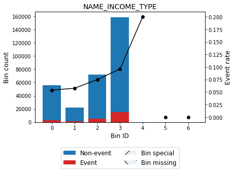
Totals		307511	1.000000	282686	24825	0.080729		0.057455	0.007146

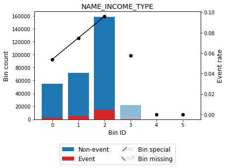
You can use the method plot to visualize the histogram and WoE or event rate curve. Note that for categorical variables the optimal bins are always monotonically ascending with respect to the event rate. Finally, note that bin 3 corresponds to bin others and is represented by using a lighter color.

[30]:

binning_table.plot(metric="event_rate")

../_images/tutorials_tutorial_binary_50_0.png

Same as for the numerical dtype, we can transform our original data into WoE or event rate values. Since version 0.17.1, if cat_unknown is None (default), transformation of unobserved categories during training follows this rule:

if transform metric == 'woe' then woe(mean event rate) = 0
if transform metric == 'event_rate' then mean event rate
if transform metric == 'indices' then -1
if transform metric == 'bins' then ‘unknown’

[31]:

x_new = ["Businessman", "Working", "New category"]

[32]:

x_transform_woe = optb.transform(x_new, metric="woe")
pd.DataFrame({variable_cat: x_new, "WoE": x_transform_woe})

[32]:

	NAME_INCOME_TYPE	WoE
0	Businessman	0.357573
1	Working	-0.188675
2	New category	0.000000

[33]:

x_transform_event_rate = optb.transform(x_new, metric="event_rate")
pd.DataFrame({variable_cat: x_new, "Event rate": x_transform_event_rate})

[33]:

	NAME_INCOME_TYPE	Event rate
0	Businessman	0.057864
1	Working	0.095885
2	New category	0.080729

[34]:

x_transform_bins = optb.transform(x_new, metric="bins")
pd.DataFrame({variable_cat: x_new, "Bin": x_transform_bins})

[34]:

	NAME_INCOME_TYPE	Bin
0	Businessman	['State servant' 'Unemployed' 'Student' 'Busin...
1	Working	['Working']
2	New category	unknown

[35]:

x_transform_indices = optb.transform(x_new, metric="indices")
pd.DataFrame({variable_cat: x_new, "Index": x_transform_indices})

[35]:

	NAME_INCOME_TYPE	Index
0	Businessman	3
1	Working	2
2	New category	-1

Advanced¶

Optimal binning Information¶

The OptimalBinning can print overview information about the options settings, problem statistics, and the solution of the computation. By default, print_level=1.

[36]:

optb = OptimalBinning(name=variable, dtype="numerical", solver="mip")
optb.fit(x, y)

[36]:

OptimalBinning(name='mean radius', solver='mip')

If print_level=0, a minimal output including the header, variable name, status, and total time are printed.

[37]:

optb.information(print_level=0)

optbinning (Version 0.19.0)
Copyright (c) 2019-2024 Guillermo Navas-Palencia, Apache License 2.0

  Name    : mean radius
  Status  : OPTIMAL

  Time    : 0.0316  sec

If print_level>=1, statistics on the pre-binning phase and the solver are printed. More detailed timing statistics are also included.

[38]:

optb.information(print_level=1)

optbinning (Version 0.19.0)
Copyright (c) 2019-2024 Guillermo Navas-Palencia, Apache License 2.0

  Name    : mean radius
  Status  : OPTIMAL

  Pre-binning statistics
    Number of pre-bins                     9
    Number of refinements                  1

  Solver statistics
    Type                                 mip
    Number of variables                   85
    Number of constraints                 45
    Objective value                   5.0439
    Best objective bound              5.0439

  Timing
    Total time                          0.03 sec
    Pre-processing                      0.00 sec   (  0.73%)
    Pre-binning                         0.00 sec   ( 10.39%)
    Solver                              0.03 sec   ( 87.59%)
    Post-processing                     0.00 sec   (  0.31%)

If print_level=2, the list of all options of the OptimalBinning are displayed. The output contains the option name, its current value and an indicator for how it was set. The unchanged options from the default settings are noted by “d”, and the options set by the user changed from the default settings are noted by “U”. This is inspired by the NAG solver e04mtc printed output, see https://www.nag.co.uk/numeric/cl/nagdoc_cl26/html/e04/e04mtc.html#fcomments.

[39]:

optb.information(print_level=2)

optbinning (Version 0.19.0)
Copyright (c) 2019-2024 Guillermo Navas-Palencia, Apache License 2.0

  Begin options
    name                         mean radius   * U
    dtype                          numerical   * d
    prebinning_method                   cart   * d
    solver                               mip   * U
    divergence                            iv   * d
    max_n_prebins                         20   * d
    min_prebin_size                     0.05   * d
    min_n_bins                            no   * d
    max_n_bins                            no   * d
    min_bin_size                          no   * d
    max_bin_size                          no   * d
    min_bin_n_nonevent                    no   * d
    max_bin_n_nonevent                    no   * d
    min_bin_n_event                       no   * d
    max_bin_n_event                       no   * d
    monotonic_trend                     auto   * d
    min_event_rate_diff                    0   * d
    max_pvalue                            no   * d
    max_pvalue_policy            consecutive   * d
    gamma                                  0   * d
    class_weight                          no   * d
    cat_cutoff                            no   * d
    cat_unknown                           no   * d
    user_splits                           no   * d
    user_splits_fixed                     no   * d
    special_codes                         no   * d
    split_digits                          no   * d
    mip_solver                           bop   * d
    time_limit                           100   * d
    verbose                            False   * d
  End options

  Name    : mean radius
  Status  : OPTIMAL

  Pre-binning statistics
    Number of pre-bins                     9
    Number of refinements                  1

  Solver statistics
    Type                                 mip
    Number of variables                   85
    Number of constraints                 45
    Objective value                   5.0439
    Best objective bound              5.0439

  Timing
    Total time                          0.03 sec
    Pre-processing                      0.00 sec   (  0.73%)
    Pre-binning                         0.00 sec   ( 10.39%)
    Solver                              0.03 sec   ( 87.59%)
    Post-processing                     0.00 sec   (  0.31%)

Binning table statistical analysis¶

The analysis method performs a statistical analysis of the binning table, computing the statistics Gini index, Information Value (IV), Jensen-Shannon divergence, and the quality score. Additionally, several statistical significance tests between consecutive bins of the contingency table are performed: a frequentist test using the Chi-square test or the Fisher’s exact test, and a Bayesian A/B test using the beta distribution as a conjugate prior of the Bernoulli distribution.

[40]:

binning_table.analysis(pvalue_test="chi2")

---------------------------------------------
OptimalBinning: Binary Binning Table Analysis
---------------------------------------------

  General metrics

    Gini index               0.12175489
    IV (Jeffrey)             0.05745546
    JS (Jensen-Shannon)      0.00714565
    Hellinger                0.00716372
    Triangular               0.02843984
    KS                       0.08364544
    HHI                      0.35824301
    HHI (normalized)         0.22989161
    Cramer's V               0.06007763
    Quality score            0.18240827

  Monotonic trend                  peak

  Significance tests

    Bin A  Bin B  t-statistic      p-value     P[A > B]  P[B > A]
        0      1   223.890188 1.281939e-50 4.799305e-71       1.0
        1      2   268.591060 2.301360e-60 6.289833e-76       1.0

[41]:

binning_table.analysis(pvalue_test="fisher")

---------------------------------------------
OptimalBinning: Binary Binning Table Analysis
---------------------------------------------

  General metrics

    Gini index               0.12175489
    IV (Jeffrey)             0.05745546
    JS (Jensen-Shannon)      0.00714565
    Hellinger                0.00716372
    Triangular               0.02843984
    KS                       0.08364544
    HHI                      0.35824301
    HHI (normalized)         0.22989161
    Cramer's V               0.06007763
    Quality score            0.18240827

  Monotonic trend                  peak

  Significance tests

    Bin A  Bin B  odd ratio      p-value     P[A > B]  P[B > A]
        0      1   1.420990 2.091361e-51 4.799305e-71       1.0
        1      2   1.310969 4.434577e-62 6.289833e-76       1.0

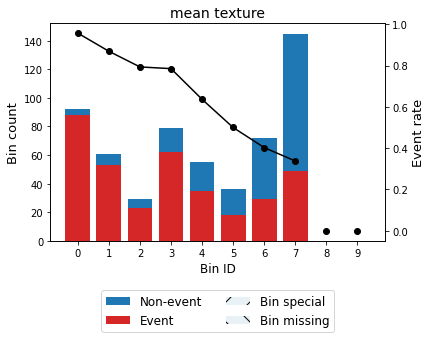
Event rate / WoE monotonicity¶

The monotonic_trend option permits forcing a monotonic trend to the event rate curve. The default setting “auto” should be the preferred option, however, some business constraints might require to impose different trends. The default setting “auto” chooses the monotonic trend most likely to maximize the information value from the options “ascending”, “descending”, “peak” and “valley” using a machine-learning-based classifier.

[42]:

variable = "mean texture"
x = df[variable].values
y = data.target

[43]:

optb = OptimalBinning(name=variable, dtype="numerical", solver="cp")
optb.fit(x, y)

[43]:

OptimalBinning(name='mean texture')

[44]:

binning_table = optb.binning_table
binning_table.build()

[44]:

	Bin	Count	Count (%)	Non-event	Event	Event rate	WoE	IV	JS
0	(-inf, 15.05)	92	0.161687	4	88	0.956522	-2.569893	0.584986	0.057939
1	[15.05, 16.39)	61	0.107206	8	53	0.868852	-1.369701	0.151658	0.017602
2	[16.39, 17.03)	29	0.050967	6	23	0.793103	-0.822585	0.029715	0.003613
3	[17.03, 18.46)	79	0.138840	17	62	0.784810	-0.772772	0.072239	0.008812
4	[18.46, 19.47)	55	0.096661	20	35	0.636364	-0.038466	0.000142	0.000018
5	[19.47, 20.20)	36	0.063269	18	18	0.500000	0.521150	0.017972	0.002221
6	[20.20, 21.71)	72	0.126538	43	29	0.402778	0.915054	0.111268	0.013443
7	[21.71, 22.74)	40	0.070299	27	13	0.325000	1.252037	0.113865	0.013371
8	[22.74, 24.00)	29	0.050967	24	5	0.172414	2.089765	0.207309	0.022035
9	[24.00, 26.98)	43	0.075571	30	13	0.302326	1.357398	0.142656	0.016578
10	[26.98, inf)	33	0.057996	15	18	0.545455	0.338828	0.006890	0.000857
11	Special	0	0.000000	0	0	0.000000	0.000000	0.000000	0.000000
12	Missing	0	0.000000	0	0	0.000000	0.000000	0.000000	0.000000
Totals		569	1.000000	212	357	0.627417		1.438701	0.156488

[45]:

binning_table.plot(metric="event_rate")

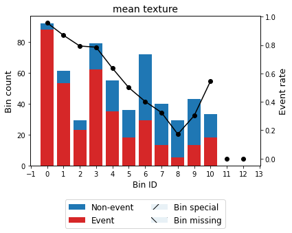
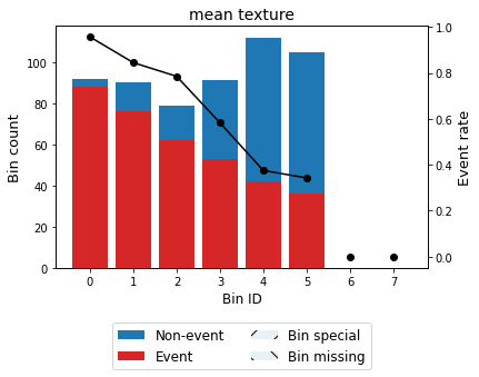
../_images/tutorials_tutorial_binary_76_0.png

For example, we can force the variable mean texture to be monotonically descending with respect to the probability of having breast cancer.

[46]:

optb = OptimalBinning(name=variable, dtype="numerical", solver="cp",
                      monotonic_trend="descending")
optb.fit(x, y)

[46]:

OptimalBinning(monotonic_trend='descending', name='mean texture')

[47]:

binning_table = optb.binning_table
binning_table.build()
binning_table.plot(metric="event_rate")

../_images/tutorials_tutorial_binary_79_0.png

Reduction of dominating bins¶

Version 0.3.0 introduced a new constraint to produce more homogeneous solutions by reducing a concentration metric such as the difference between the largest and smallest bin. The added regularization parameter gamma controls the importance of the reduction term. Larger values specify stronger regularization. Continuing with the previous example

[48]:

optb = OptimalBinning(name=variable, dtype="numerical", solver="cp",
                      monotonic_trend="descending", gamma=0.5)
optb.fit(x, y)

[48]:

OptimalBinning(gamma=0.5, monotonic_trend='descending', name='mean texture')

[49]:

binning_table = optb.binning_table
binning_table.build()
binning_table.plot(metric="event_rate")

../_images/tutorials_tutorial_binary_83_0.png

Note that the new solution produces more homogeneous bins, removing the dominance of bin 7 previously observed.

User-defined split points¶

In some situations, we have defined split points or bins required to satisfy a priori belief, knowledge or business constraint. The OptimalBinning permits to pass user-defined split points for numerical variables and user-defined bins for categorical variables. The supplied information is used as a pre-binning, disallowing any pre-binning method set by the user. Furthermore, version 0.5.0 introduces user_splits_fixed parameter, to allow the user to fix some user-defined splits, so these must appear in the solution.

Example numerical variable:

[50]:

user_splits =       [  14,    15,    16,    17,    20,    21,    22,    27]
user_splits_fixed = [False, True,  True, False, False, False, False, False]

[51]:

optb = OptimalBinning(name=variable, dtype="numerical", solver="mip",
                      user_splits=user_splits, user_splits_fixed=user_splits_fixed)

optb.fit(x, y)

[51]:

OptimalBinning(name='mean texture', solver='mip',
               user_splits=[14, 15, 16, 17, 20, 21, 22, 27],
               user_splits_fixed=array([False,  True,  True, False, False, False, False, False]))

[52]:

binning_table = optb.binning_table
binning_table.build()

[52]:

	Bin	Count	Count (%)	Non-event	Event	Event rate	WoE	IV	JS
0	(-inf, 14.00)	54	0.094903	2	52	0.962963	-2.736947	0.372839	0.035974
1	[14.00, 15.00)	37	0.065026	2	35	0.945946	-2.341051	0.207429	0.021268
2	[15.00, 16.00)	43	0.075571	7	36	0.837209	-1.116459	0.075720	0.009002
3	[16.00, 20.00)	210	0.369069	59	151	0.719048	-0.418593	0.060557	0.007515
4	[20.00, 21.00)	45	0.079086	26	19	0.422222	0.834807	0.057952	0.007041
5	[21.00, 22.00)	49	0.086116	30	19	0.387755	0.977908	0.086338	0.010382
6	[22.00, 27.00)	99	0.173989	71	28	0.282828	1.451625	0.372304	0.042839
7	[27.00, inf)	32	0.056239	15	17	0.531250	0.395986	0.009161	0.001138
8	Special	0	0.000000	0	0	0.000000	0.000000	0.000000	0.000000
9	Missing	0	0.000000	0	0	0.000000	0.000000	0.000000	0.000000
Totals		569	1.000000	212	357	0.627417		1.242301	0.135158

[53]:

optb.information()

optbinning (Version 0.19.0)
Copyright (c) 2019-2024 Guillermo Navas-Palencia, Apache License 2.0

  Name    : mean texture
  Status  : OPTIMAL

  Pre-binning statistics
    Number of pre-bins                     9
    Number of refinements                  0

  Solver statistics
    Type                                 mip
    Number of variables                  137
    Number of constraints                 55
    Objective value                   1.2423
    Best objective bound              1.2423

  Timing
    Total time                          0.07 sec
    Pre-processing                      0.00 sec   (  0.26%)
    Pre-binning                         0.00 sec   (  1.50%)
    Solver                              0.07 sec   ( 97.15%)
    Post-processing                     0.00 sec   (  0.18%)

Example categorical variable:

[54]:

user_splits = np.array([
               ['Businessman'],
               ['Working'],
               ['Commercial associate'],
               ['Pensioner', 'Maternity leave'],
               ['State servant'],
               ['Unemployed', 'Student']], dtype=object)

[55]:

optb = OptimalBinning(name=variable_cat, dtype="categorical", solver="cp",
                      user_splits=user_splits,
                      user_splits_fixed=[False, True, True, True, True, True])

optb.fit(x_cat, y_cat)

[55]:

OptimalBinning(dtype='categorical', name='NAME_INCOME_TYPE',
               user_splits=array([list(['Working']), list(['Commercial associate']),
       list(['Pensioner', 'Maternity leave']), list(['State servant']),
       list(['Unemployed', 'Student'])], dtype=object),
               user_splits_fixed=array([ True,  True,  True,  True,  True]))

[56]:

binning_table = optb.binning_table
binning_table.build()

[56]:

	Bin	Count	Count (%)	Non-event	Event	Event rate	WoE	IV	JS
0	[Businessman, Pensioner, Maternity leave]	55377	0.180081	52393	2984	0.053885	0.433023	0.028206	0.003499
1	[State servant]	21703	0.070576	20454	1249	0.057550	0.363350	0.008010	0.000996
2	[Commercial associate]	71617	0.232892	66257	5360	0.074843	0.082092	0.001516	0.000189
3	[Working]	158774	0.516320	143550	15224	0.095885	-0.188675	0.019895	0.002483
4	[Unemployed, Student]	40	0.000130	32	8	0.200000	-1.046191	0.000219	0.000026
5	Special	0	0.000000	0	0	0.000000	0.000000	0.000000	0.000000
6	Missing	0	0.000000	0	0	0.000000	0.000000	0.000000	0.000000
Totals		307511	1.000000	282686	24825	0.080729		0.057846	0.007193

[57]:

optb.binning_table.plot(metric="event_rate")

../_images/tutorials_tutorial_binary_96_0.png

[58]:

optb.information()

optbinning (Version 0.19.0)
Copyright (c) 2019-2024 Guillermo Navas-Palencia, Apache License 2.0

  Name    : NAME_INCOME_TYPE
  Status  : OPTIMAL

  Pre-binning statistics
    Number of pre-bins                     5
    Number of refinements                  1

  Solver statistics
    Type                                  cp
    Number of booleans                     0
    Number of branches                     0
    Number of conflicts                    0
    Objective value                    57843
    Best objective bound               57843

  Timing
    Total time                          0.28 sec
    Pre-processing                      0.04 sec   ( 16.31%)
    Pre-binning                         0.22 sec   ( 79.89%)
    Solver                              0.01 sec   (  3.57%)
      model generation                  0.01 sec   ( 87.30%)
      optimizer                         0.00 sec   ( 12.70%)
    Post-processing                     0.00 sec   (  0.02%)

Performance: choosing a solver¶

For small problems, say less than max_n_prebins<=20, the solver="mip" tends to be faster than solver="cp". However, for medium and large problems, experiments show the contrary. For very large problems, we recommend the use of the commercial solver LocalSolver via solver="ls". See the specific LocalSolver tutorial.

Missing data and special codes¶

For this example, let’s load data from the FICO Explainable Machine Learning Challenge: https://community.fico.com/s/explainable-machine-learning-challenge

[59]:

df = pd.read_csv("data/FICO_challenge/heloc_dataset_v1.csv", sep=",")

The data dictionary of this challenge includes three special values/codes:

-9 No Bureau Record or No Investigation
-8 No Usable/Valid Trades or Inquiries
-7 Condition not Met (e.g. No Inquiries, No Delinquencies)

[60]:

special_codes = [-9, -8, -7]

[61]:

variable = "AverageMInFile"
x = df[variable].values
y = df.RiskPerformance.values

[62]:

df.RiskPerformance.unique()

[62]:

array(['Bad', 'Good'], dtype=object)

Target is a categorical dichotomic variable, which can be easily transform into numerical.

[63]:

mask = y == "Bad"
y[mask] = 1
y[~mask] = 0
y = y.astype(int)

For the sake of completeness, we include a few missing values

[64]:

idx = np.random.randint(0, len(x), 500)
x = x.astype(float)
x[idx] = np.nan

[65]:

optb = OptimalBinning(name=variable, dtype="numerical", solver="mip",
                      special_codes=special_codes)

optb.fit(x, y)

[65]:

OptimalBinning(name='AverageMInFile', solver='mip', special_codes=[-9, -8, -7])

[66]:

optb.information(print_level=1)

optbinning (Version 0.19.0)
Copyright (c) 2019-2024 Guillermo Navas-Palencia, Apache License 2.0

  Name    : AverageMInFile
  Status  : OPTIMAL

  Pre-binning statistics
    Number of pre-bins                    13
    Number of refinements                  0

  Solver statistics
    Type                                 mip
    Number of variables                  174
    Number of constraints                 91
    Objective value                   0.3235
    Best objective bound              0.3235

  Timing
    Total time                          0.10 sec
    Pre-processing                      0.00 sec   (  3.77%)
    Pre-binning                         0.01 sec   (  8.61%)
    Solver                              0.09 sec   ( 86.93%)
    Post-processing                     0.00 sec   (  0.11%)

[67]:

binning_table = optb.binning_table
binning_table.build()

[67]:

	Bin	Count	Count (%)	Non-event	Event	Event rate	WoE	IV	JS
0	(-inf, 30.50)	549	0.052491	98	451	0.821494	-1.438672	0.090659	0.010446
1	[30.50, 48.50)	1044	0.099818	286	758	0.726054	-0.886864	0.072415	0.008766
2	[48.50, 56.50)	698	0.066737	248	450	0.644699	-0.507991	0.016679	0.002063
3	[56.50, 64.50)	928	0.088727	389	539	0.580819	-0.238309	0.004989	0.000622
4	[64.50, 69.50)	661	0.063199	301	360	0.544629	-0.091166	0.000524	0.000065
5	[69.50, 74.50)	679	0.064920	327	352	0.518409	0.014157	0.000013	0.000002
6	[74.50, 81.50)	901	0.086146	466	435	0.482797	0.156667	0.002117	0.000264
7	[81.50, 101.50)	1987	0.189980	1129	858	0.431807	0.362311	0.024865	0.003091
8	[101.50, 116.50)	865	0.082704	540	325	0.375723	0.595572	0.028865	0.003556
9	[116.50, inf)	1089	0.104121	706	383	0.351699	0.699408	0.049686	0.006087
10	Special	565	0.054020	253	312	0.552212	-0.121786	0.000798	0.000100
11	Missing	493	0.047136	257	236	0.478702	0.173072	0.001414	0.000177
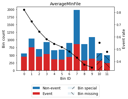
Totals		10459	1.000000	5000	5459	0.521943		0.293024	0.035239

Note the dashed bins 10 and 11, corresponding to the special codes bin and the missing bin, respectively.

[68]:

binning_table.plot(metric="event_rate")

../_images/tutorials_tutorial_binary_115_0.png

Treat special codes separately¶

Version 0.13.0 introduced the option to pass a dictionary of special codes to treat them separately. This feature provides more flexibility to the modeller. Note that a special code can be a single value or a list of values, for example, a combination of several special values.

[69]:

special_codes = {'special_1': -9, "special_2": -8, "special_3": -7}

x[10:20] = -8
x[100:105] = -7

optb = OptimalBinning(name=variable, dtype="numerical", solver="mip",
                      special_codes=special_codes)

optb.fit(x, y)

[69]:

OptimalBinning(name='AverageMInFile', solver='mip',
               special_codes={'special_1': -9, 'special_2': -8,
                              'special_3': -7})

[70]:

optb.binning_table.build()

[70]:

	Bin	Count	Count (%)	Non-event	Event	Event rate	WoE	IV	JS
0	(-inf, 30.50)	548	0.052395	98	450	0.821168	-1.436452	0.090256	0.010402
1	[30.50, 48.50)	1042	0.099627	285	757	0.726488	-0.889046	0.072608	0.008788
2	[48.50, 56.50)	698	0.066737	248	450	0.644699	-0.507991	0.016679	0.002063
3	[56.50, 64.50)	927	0.088632	389	538	0.580367	-0.236452	0.004907	0.000612
4	[64.50, 69.50)	658	0.062912	301	357	0.542553	-0.082798	0.000430	0.000054
5	[69.50, 74.50)	679	0.064920	327	352	0.518409	0.014157	0.000013	0.000002
6	[74.50, 81.50)	899	0.085955	466	433	0.481646	0.161276	0.002239	0.000280
7	[81.50, 101.50)	1984	0.189693	1128	856	0.431452	0.363759	0.025025	0.003111
8	[101.50, 116.50)	865	0.082704	540	325	0.375723	0.595572	0.028865	0.003556
9	[116.50, inf)	1087	0.103930	705	382	0.351426	0.700605	0.049760	0.006096
10	special_1	565	0.054020	253	312	0.552212	-0.121786	0.000798	0.000100
11	special_2	10	0.000956	2	8	0.800000	-1.298467	0.001383	0.000162
12	special_3	5	0.000478	2	3	0.600000	-0.317637	0.000048	0.000006
13	Missing	492	0.047041	256	236	0.479675	0.169173	0.001348	0.000168
Totals		10459	1.000000	5000	5459	0.521943		0.294358	0.035398

[71]:

optb.binning_table.plot(metric="event_rate")

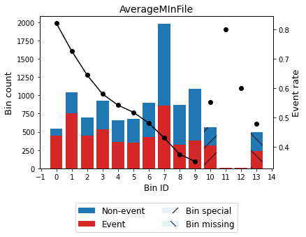
../_images/tutorials_tutorial_binary_120_0.png

[72]:

special_codes = {'special_1': -9, "special_comb": [-7, -8]}

optb = OptimalBinning(name=variable, dtype="numerical", solver="mip",
                      special_codes=special_codes)

optb.fit(x, y)

[72]:

OptimalBinning(name='AverageMInFile', solver='mip',
               special_codes={'special_1': -9, 'special_comb': [-7, -8]})

[73]:

optb.binning_table.build()

[73]:

	Bin	Count	Count (%)	Non-event	Event	Event rate	WoE	IV	JS
0	(-inf, 30.50)	548	0.052395	98	450	0.821168	-1.436452	0.090256	0.010402
1	[30.50, 48.50)	1042	0.099627	285	757	0.726488	-0.889046	0.072608	0.008788
2	[48.50, 56.50)	698	0.066737	248	450	0.644699	-0.507991	0.016679	0.002063
3	[56.50, 64.50)	927	0.088632	389	538	0.580367	-0.236452	0.004907	0.000612
4	[64.50, 69.50)	658	0.062912	301	357	0.542553	-0.082798	0.000430	0.000054
5	[69.50, 74.50)	679	0.064920	327	352	0.518409	0.014157	0.000013	0.000002
6	[74.50, 81.50)	899	0.085955	466	433	0.481646	0.161276	0.002239	0.000280
7	[81.50, 101.50)	1984	0.189693	1128	856	0.431452	0.363759	0.025025	0.003111
8	[101.50, 116.50)	865	0.082704	540	325	0.375723	0.595572	0.028865	0.003556
9	[116.50, inf)	1087	0.103930	705	382	0.351426	0.700605	0.049760	0.006096
10	special_1	565	0.054020	253	312	0.552212	-0.121786	0.000798	0.000100
11	special_comb	15	0.001434	4	11	0.733333	-0.923773	0.001122	0.000136
12	Missing	492	0.047041	256	236	0.479675	0.169173	0.001348	0.000168
Totals		10459	1.000000	5000	5459	0.521943		0.294050	0.035366

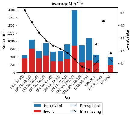
Version 0.15.1 added the option show_bin_labels to show the bin label instead of the bin id on the x-axis.

[74]:

optb.binning_table.plot(metric="event_rate", show_bin_labels=True)

../_images/tutorials_tutorial_binary_124_0.png

Verbosity option¶

For debugging purposes, we can print information on each step of the computation by triggering the verbose option.

[75]:

optb = OptimalBinning(name=variable, dtype="numerical", solver="mip", verbose=True)
optb.fit(x, y)

2024-01-14 23:33:34,971 | INFO : Optimal binning started.
2024-01-14 23:33:34,973 | INFO : Options: check parameters.
2024-01-14 23:33:34,976 | INFO : Pre-processing started.
2024-01-14 23:33:34,977 | INFO : Pre-processing: number of samples: 10459
2024-01-14 23:33:34,981 | INFO : Pre-processing: number of clean samples: 9967
2024-01-14 23:33:34,982 | INFO : Pre-processing: number of missing samples: 492
2024-01-14 23:33:34,984 | INFO : Pre-processing: number of special samples: 0
2024-01-14 23:33:34,985 | INFO : Pre-processing terminated. Time: 0.0021s
2024-01-14 23:33:34,987 | INFO : Pre-binning started.
2024-01-14 23:33:35,003 | INFO : Pre-binning: number of prebins: 15
2024-01-14 23:33:35,004 | INFO : Pre-binning: number of refinements: 0
2024-01-14 23:33:35,005 | INFO : Pre-binning terminated. Time: 0.0144s
2024-01-14 23:33:35,006 | INFO : Optimizer started.
2024-01-14 23:33:35,008 | INFO : Optimizer: classifier predicts descending monotonic trend.
2024-01-14 23:33:35,010 | INFO : Optimizer: monotonic trend set to descending.
2024-01-14 23:33:35,011 | INFO : Optimizer: build model...
2024-01-14 23:33:35,122 | INFO : Optimizer: solve...
2024-01-14 23:33:35,126 | INFO : Optimizer terminated. Time: 0.1194s
2024-01-14 23:33:35,128 | INFO : Post-processing started.
2024-01-14 23:33:35,130 | INFO : Post-processing: compute binning information.
2024-01-14 23:33:35,133 | INFO : Post-processing terminated. Time: 0.0002s
2024-01-14 23:33:35,135 | INFO : Optimal binning terminated. Status: OPTIMAL. Time: 0.1640s

[75]:

OptimalBinning(name='AverageMInFile', solver='mip', verbose=True)