Optimal binning for streaming data

The optimal binning is the constrained discretization of a numerical feature into bins given a binary target, maximizing a statistic such as Jeffrey's divergence or Gini. Binning is a data preprocessing technique commonly used in binary classification, but the current list of existing binning algorithms supporting constraints lacks a method to handle streaming data. In this post, I propose a new scalable, memory-efficient and robust algorithm for performing optimal binning in the streaming settings. The described algorithm will be implemented in the open-source python library OptBinning version 0.7.0.

The following image shows how the optimal binning is dynamically updated as new data arrives. Note that the number of abrupt changes diminishes when the number of records increases, obtaining a more stable solution.

Algorithm: binning sketch

The proposed optimal binning process comprises two steps: A pre-binning process that generates an initial granular discretization, and a subsequent optimization to satisfy imposed constraints. The pre-binning process might use unsupervised techniques such as equal-width and equal-size or equal-frequency interval binning, or supervised algorithms such as a decision tree algorithm to calculate the initial split points. The resulting \(m\) split points are sorted in strictly ascending order, \(s_1 < s_2 < \ldots < s_m\) to create \(n = m + 1\) pre-bins. These pre-bins are defined by the intervals \((-\infty, s_1), [s_1, s_2), \ldots, [s_m, \infty)\). Given a binary target \(y\) used to discretize a variable \(x\) into \(n\) bins, the normalized count of non-events (NE) \(p_i\) and events (E) \(q_i\) for each bin \(i\) are defined as $$p_i = \frac{r_i^{NE}}{r_T^{NE}}, \quad q_i = \frac{r_i^E}{r_T^E},$$ where \(r_T^{NE}\) and \(r_T^E\) are the total number of non-event records and event records, respectively.

The binning sketch algorithm is used as a pre-binning method of the optimal binning algorithm for data streams. The algorithm and underlying data structure is based on quantile sketching algorithms. The best known rank-error quantile sketch is the Greenwald-Khanna's deterministic quantiles sketch (GK) M. Greenwald and S. Khanna, "Space-Efficient Online Computation of Quantile Summaries", 2001. GK computes \(\epsilon\) accuracy quantiles with worst-case space \(O((1/\epsilon)\log(\epsilon n))\) for \(n\) elements (a variation of GK is implemented in Apache Spark function approxQuantile). A recent algorithm exhibiting higher relative accuracy is t-digest, "T. Dunning and O. Ertl, "Computing Extremely Accurate Quantiles Using t-Digests", 2019. For this work, both sketch algorithms are considered, but only the t-digest algorithm is discussed in detail.

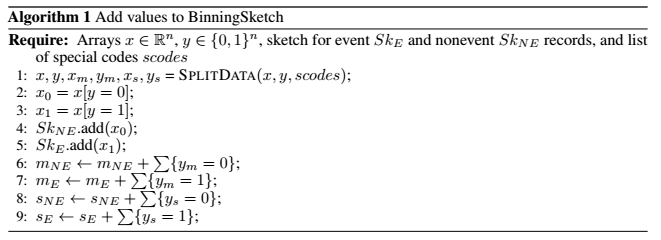
The first step is splitting data into three subsets \([(x, y), (x_m, y_m), (x_s, y_s)]\) corresponding to clean, missing and special codes data, respectively. At the same time, the number of non-event and event records is stored in the binning sketch data structure. See Algorithm 1.

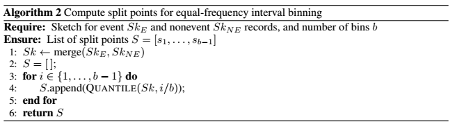
The binning sketch algorithm performs the pre-binning process using equal-frequency interval binning. To do so, first, the internal sketch corresponding to event and non-event records are combined (mergeability) as a single sketch accounting for all data. Subsequently, \(b - 1\) quantiles (split points \(s\)) are computed to generate \(b\) pre-bins. This step is described in Algorithm 2.

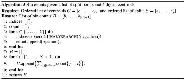
The last step is to compute the bin counts for event and non-event. The procedure devised for t-digest is described in Algorithm 3. The number of event and non-event records for each pre-bin is the number of elements of the centroid which mean value is within the computed \(b\) intervals.

Once the pre-bins are computed, the optimal binning algorithm is solved using the mixed-integer programming formulation or constraint programming formulation described in G. Navas-Palencia "Optimal binning: mathematical programming formulation", 2020. The formulation is a generalized assignment problem with several special constraints. The average CPU time for instances with approximately 20 pre-bins is in the order of milliseconds. Consequently, online optimal binning is feasible, permitting its usage in applications requiring near real-time monitoring of data streams.

Experiments

The following tables show the accuracy of the proposed approach on a selection of variables from the public dataset Home Credit Default Risk - Kaggle’s competition. This dataset contains 307511 samples.The experiments were run on Intel(R) Core(TM) i5-3317 CPU at 1.70GHz, using a single core, running Linux. The optimal IV is computed using OptimalBinning with equal-frequency (quantile) pre-bins, and minimum bin size 5%.

optb = OptimalBinning(prebinning_method="quantile", min_bin_size=0.05)
optb.fit(x, y)

The optimal binning algorithm with data streams is implemented in a new class OptimalBinningSketch. For these experiments, I use partitions of varying sizes from the selected dataset to simulate data streams. Note that this algorithm is also suitable to be implemented in Spark via mapPartitions. An implementation using pandas.read_csv by chunks is given below,

def add(chunk):
    x = chunk[variable].values
    y = chunk[target].values
   
    optbsketch = OptimalBinningSketch(eps=0.001, sketch="t-digest", min_bin_size=0.05)
    optbsketch.add(x, y)
    
    return optbsketch
    
def merge(optbsketch, other_optbsketch):
    optbsketch.merge(other_optbsketch)
    
    return optbsketch

# MapReduce structure:
chunks = pd.read_csv(filepath_or_buffer=filepath, engine='c', chunksize=100,
                     usecols=[variable, target])

optbsketch = reduce(merge, map(add, chunks))	

optbsketch.solve()

Experiment 1: Variable AMT_INCOME_TOTAL. Optimal IV using the complete dataset is 0.011161 with 9 bins.

A) Quantile sketch algorithm: GK with absolute error 0.0001 (0.1%):

Chunk size	IV	# Bins	Error
10	0.010946	9	1.93%
100	0.011018	9	1.28%
1000	0.010941	9	1.97%
10000	0.011418	9	2.30%

B) Quantile sketch algorithm: t-digest with relative error 0.0001 (0.1%):

Chunk size	IV	# Bins	Error
1000	0.011117	9	0.40%
10000	0.011074	8	0.78%

Experiment 2: Variable EXT_SOURCE_2. Optimal IV using the complete dataset is 0.30649 with 10 bins. This variable contains missing values.

A) Quantile sketch algorithm: GK with absolute error 0.0001 (0.1%):

Chunk size	IV	# Bins	Error
10	0.314964	11	2.76%
100	0.315855	12	3.06%
1000	0.315473	10	2.93%
10000	0.315995	11	3.10%

B) Quantile sketch algorithm: t-digest with relative error 0.0001 (0.1%):

Chunk size	IV	# Bins	Error
1000	0.306903	10	0.13%
10000	0.306083	10	0.13%

Both quantile sketch algorithms produce good results, being the t-digest the most accurate. The t-digest algorithm implementation https://github.com/CamDavidsonPilon/tdigest is significantly slower than the GK implementation based on https://github.com/DataDog/sketches-py/tree/master/gkarray, thus, GK is the recommended algorithm when handling partitions. Besides, GK is deterministic, therefore returning reproducible results.