Tutorial: Telco customer churn
In this tutorial, we use the dataset form the Kaggle competition: https://www.kaggle.com/blastchar/telco-customer-churn. The goal of the challenge is to predict behavior to retain customers by analyzing all relevant customer data and developing focused customer retention programs.
[1]:
import numpy as np
import pandas as pd

from optbinning import BinningProcess
Download the dataset from the link above and load it.
[2]:
df = pd.read_csv("data/kaggle/WA_Fn-UseC_-Telco-Customer-Churn.csv", sep=",", engine="c")
[3]:
df.head()
[3]:
| customerID | gender | SeniorCitizen | Partner | Dependents | tenure | PhoneService | MultipleLines | InternetService | OnlineSecurity | ... | DeviceProtection | TechSupport | StreamingTV | StreamingMovies | Contract | PaperlessBilling | PaymentMethod | MonthlyCharges | TotalCharges | Churn | |
|---|---|---|---|---|---|---|---|---|---|---|---|---|---|---|---|---|---|---|---|---|---|
| 0 | 7590-VHVEG | Female | 0 | Yes | No | 1 | No | No phone service | DSL | No | ... | No | No | No | No | Month-to-month | Yes | Electronic check | 29.85 | 29.85 | No |
| 1 | 5575-GNVDE | Male | 0 | No | No | 34 | Yes | No | DSL | Yes | ... | Yes | No | No | No | One year | No | Mailed check | 56.95 | 1889.50 | No |
| 2 | 3668-QPYBK | Male | 0 | No | No | 2 | Yes | No | DSL | Yes | ... | No | No | No | No | Month-to-month | Yes | Mailed check | 53.85 | 108.15 | Yes |
| 3 | 7795-CFOCW | Male | 0 | No | No | 45 | No | No phone service | DSL | Yes | ... | Yes | Yes | No | No | One year | No | Bank transfer (automatic) | 42.30 | 1840.75 | No |
| 4 | 9237-HQITU | Female | 0 | No | No | 2 | Yes | No | Fiber optic | No | ... | No | No | No | No | Month-to-month | Yes | Electronic check | 70.70 | 151.65 | Yes |
5 rows × 21 columns
For this tutorial we use a pandas.Dataframe as input, option supported since version 0.4.0.
[4]:
variable_names = list(df.columns[:-1])

X = df[variable_names]
y = df["Churn"].values
Transform the categorical dichotomic target variable into numerical.
[5]:
mask = y == "Yes"
y[mask] = 1
y[~mask] = 0
y = y.astype(int)
The dichotomic variable SeniorCitizen is treated as nominal (categorical).
[6]:
categorical_variables = ["SeniorCitizen"]
Instantiate a BinningProcess object class with variable names and the list of numerical variables to be considered categorical. Fit with dataframe X and target array y.
Variable selection criteria
Using parameter selection_criteria, we specify the criteria for variable selection. These criteria will select the top 10 highest IV variables with IV in [0.025, 0.7] and quality score >= 0.01 to discard non-predictive and low-quality variables.
[7]:
selection_criteria = {
    "iv": {"min": 0.025, "max": 0.7, "strategy": "highest", "top": 10},
    "quality_score": {"min": 0.01}
}
[8]:
binning_process = BinningProcess(variable_names,
                                 categorical_variables=categorical_variables,
                                 selection_criteria=selection_criteria)
binning_process.fit(X, y)
[8]:
BinningProcess(categorical_variables=['SeniorCitizen'],
               selection_criteria={'iv': {'max': 0.7, 'min': 0.025,
                                          'strategy': 'highest', 'top': 10},
                                   'quality_score': {'min': 0.01}},
               variable_names=['customerID', 'gender', 'SeniorCitizen',
                               'Partner', 'Dependents', 'tenure',
                               'PhoneService', 'MultipleLines',
                               'InternetService', 'OnlineSecurity',
                               'OnlineBackup', 'DeviceProtection',
                               'TechSupport', 'StreamingTV', 'StreamingMovies',
                               'Contract', 'PaperlessBilling', 'PaymentMethod',
                               'MonthlyCharges', 'TotalCharges'])
Binning process statistics
The binning process of the pipeline can be retrieved to show information about the problem and timing statistics.
[9]:
binning_process.information(print_level=2)
optbinning (Version 0.19.0)
Copyright (c) 2019-2024 Guillermo Navas-Palencia, Apache License 2.0

  Begin options
    max_n_prebins                         20   * d
    min_prebin_size                     0.05   * d
    min_n_bins                            no   * d
    max_n_bins                            no   * d
    min_bin_size                          no   * d
    max_bin_size                          no   * d
    max_pvalue                            no   * d
    max_pvalue_policy            consecutive   * d
    selection_criteria                   yes   * U
    fixed_variables                       no   * d
    categorical_variables                yes   * U
    special_codes                         no   * d
    split_digits                          no   * d
    binning_fit_params                    no   * d
    binning_transform_params              no   * d
    verbose                            False   * d
  End options

  Statistics
    Number of records                   7043
    Number of variables                   20
    Target type                       binary

    Number of numerical                    3
    Number of categorical                 17
    Number of selected                    10

  Time                                1.1470 sec
The summary method returns basic statistics for each binned variable.
[10]:
binning_process.summary()
[10]:
| name | dtype | status | selected | n_bins | iv | js | gini | quality_score | |
|---|---|---|---|---|---|---|---|---|---|
| 0 | customerID | categorical | OPTIMAL | False | 1 | 0.000000 | 0.000000 | 0 | 0.000000 |
| 1 | gender | categorical | OPTIMAL | False | 2 | 0.000380 | 0.000048 | 0.009752 | 0.000560 |
| 2 | SeniorCitizen | categorical | OPTIMAL | False | 2 | 0.105621 | 0.012996 | 0.125961 | 0.153839 |
| 3 | Partner | categorical | OPTIMAL | False | 2 | 0.118729 | 0.014763 | 0.170273 | 0.314888 |
| 4 | Dependents | categorical | OPTIMAL | False | 2 | 0.155488 | 0.019151 | 0.170376 | 0.335552 |
| 5 | tenure | numerical | OPTIMAL | False | 11 | 0.872052 | 0.097305 | 0.481435 | 0.056737 |
| 6 | PhoneService | categorical | OPTIMAL | False | 2 | 0.000745 | 0.000093 | 0.007999 | 0.000495 |
| 7 | MultipleLines | categorical | OPTIMAL | False | 3 | 0.008207 | 0.001025 | 0.045135 | 0.001278 |
| 8 | InternetService | categorical | OPTIMAL | True | 3 | 0.617953 | 0.073195 | 0.390396 | 0.610141 |
| 9 | OnlineSecurity | categorical | OPTIMAL | False | 3 | 0.717777 | 0.085303 | 0.410962 | 0.450406 |
| 10 | OnlineBackup | categorical | OPTIMAL | True | 3 | 0.528634 | 0.062309 | 0.355336 | 0.724060 |
| 11 | DeviceProtection | categorical | OPTIMAL | True | 3 | 0.499725 | 0.058772 | 0.341513 | 0.752393 |
| 12 | TechSupport | categorical | OPTIMAL | True | 3 | 0.699567 | 0.083122 | 0.406944 | 0.477804 |
| 13 | StreamingTV | categorical | OPTIMAL | True | 3 | 0.380462 | 0.044117 | 0.239797 | 0.801691 |
| 14 | StreamingMovies | categorical | OPTIMAL | True | 3 | 0.381374 | 0.044229 | 0.242055 | 0.804383 |
| 15 | Contract | categorical | OPTIMAL | False | 3 | 1.238560 | 0.134486 | 0.478217 | 0.028676 |
| 16 | PaperlessBilling | categorical | OPTIMAL | True | 2 | 0.203068 | 0.025087 | 0.213501 | 0.477619 |
| 17 | PaymentMethod | categorical | OPTIMAL | True | 4 | 0.457109 | 0.055846 | 0.342473 | 0.585114 |
| 18 | MonthlyCharges | numerical | OPTIMAL | True | 5 | 0.376524 | 0.044813 | 0.288365 | 0.381020 |
| 19 | TotalCharges | numerical | OPTIMAL | True | 10 | 0.354844 | 0.042627 | 0.319420 | 0.034886 |
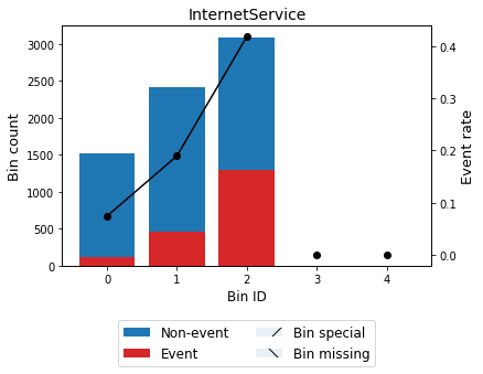
The get_binned_variable method serves to retrieve an optimal binning object, which can be analyzed in detail afterward. Let us analyze the variable “InternetService” representing the customer’s internet service provider (DSL, Fiber optic, No). We observe that customers with Fiber optic internet service providers are more likely to churn.
[11]:
optb = binning_process.get_binned_variable("InternetService")
optb.binning_table.build()
[11]:
| Bin | Count | Count (%) | Non-event | Event | Event rate | WoE | IV | JS | |
|---|---|---|---|---|---|---|---|---|---|
| 0 | [No] | 1526 | 0.216669 | 1413 | 113 | 0.074050 | 1.507840 | 0.320621 | 0.036666 |
| 1 | [DSL] | 2421 | 0.343746 | 1962 | 459 | 0.189591 | 0.434427 | 0.058047 | 0.007199 |
| 2 | [Fiber optic] | 3096 | 0.439585 | 1799 | 1297 | 0.418928 | -0.691066 | 0.239284 | 0.029329 |
| 3 | Special | 0 | 0.000000 | 0 | 0 | 0.000000 | 0.000000 | 0.000000 | 0.000000 |
| 4 | Missing | 0 | 0.000000 | 0 | 0 | 0.000000 | 0.000000 | 0.000000 | 0.000000 |
| Totals | 7043 | 1.000000 | 5174 | 1869 | 0.265370 | 0.617953 | 0.073195 |
[12]:
optb.binning_table.plot(metric="event_rate")
Now, we analyze variable “tenure” representing the number of months the customer has stayed with the company. We see a notorious descending trend indicating that the probability of churn decreases as the permanence of the contract increases.
[13]:
optb = binning_process.get_binned_variable("tenure")
optb.binning_table.build()
[13]:
| Bin | Count | Count (%) | Non-event | Event | Event rate | WoE | IV | JS | |
|---|---|---|---|---|---|---|---|---|---|
| 0 | (-inf, 1.50) | 624 | 0.088599 | 244 | 380 | 0.608974 | -1.461246 | 0.228186 | 0.026229 |
| 1 | [1.50, 5.50) | 747 | 0.106063 | 383 | 364 | 0.487282 | -0.967361 | 0.116792 | 0.014055 |
| 2 | [5.50, 10.50) | 599 | 0.085049 | 375 | 224 | 0.373957 | -0.502963 | 0.023827 | 0.002947 |
| 3 | [10.50, 16.50) | 580 | 0.082351 | 384 | 196 | 0.337931 | -0.345715 | 0.010597 | 0.001318 |
| 4 | [16.50, 22.50) | 481 | 0.068295 | 350 | 131 | 0.272349 | -0.035507 | 0.000087 | 0.000011 |
| 5 | [22.50, 33.50) | 808 | 0.114724 | 629 | 179 | 0.221535 | 0.238503 | 0.006152 | 0.000767 |
| 6 | [33.50, 43.50) | 647 | 0.091864 | 512 | 135 | 0.208655 | 0.314807 | 0.008413 | 0.001047 |
| 7 | [43.50, 49.50) | 384 | 0.054522 | 322 | 62 | 0.161458 | 0.629175 | 0.018285 | 0.002249 |
| 8 | [49.50, 59.50) | 690 | 0.097970 | 591 | 99 | 0.143478 | 0.768454 | 0.047072 | 0.005743 |
| 9 | [59.50, 70.50) | 951 | 0.135028 | 864 | 87 | 0.091483 | 1.277422 | 0.153853 | 0.018022 |
| 10 | [70.50, inf) | 532 | 0.075536 | 520 | 12 | 0.022556 | 2.750680 | 0.258789 | 0.024916 |
| 11 | Special | 0 | 0.000000 | 0 | 0 | 0.000000 | 0.000000 | 0.000000 | 0.000000 |
| 12 | Missing | 0 | 0.000000 | 0 | 0 | 0.000000 | 0.000000 | 0.000000 | 0.000000 |
| Totals | 7043 | 1.000000 | 5174 | 1869 | 0.265370 | 0.872052 | 0.097305 |
[14]:
optb.binning_table.plot(metric="event_rate")

Transformation
Let’s check the selected variables with the given selection criteria.
[15]:
binning_process.get_support(names=True)
[15]:
array(['InternetService', 'OnlineBackup', 'DeviceProtection',
       'TechSupport', 'StreamingTV', 'StreamingMovies',
       'PaperlessBilling', 'PaymentMethod', 'MonthlyCharges',
       'TotalCharges'], dtype='<U16')
Now we transform the original dataset to Weight of Evidence. Only the selected variables will be included in the transformed dataframe.
[16]:
X_transform = binning_process.transform(X, metric="woe")
[17]:
X_transform
[17]:
| InternetService | OnlineBackup | DeviceProtection | TechSupport | StreamingTV | StreamingMovies | PaperlessBilling | PaymentMethod | MonthlyCharges | TotalCharges | |
|---|---|---|---|---|---|---|---|---|---|---|
| 0 | 0.434427 | 0.274938 | -0.576292 | -0.680487 | -0.333624 | -0.340675 | -0.335507 | -0.829097 | 0.202003 | -1.158825 |
| 1 | 0.434427 | -0.609808 | 0.218402 | -0.680487 | -0.333624 | -0.340675 | 0.615628 | 0.424849 | 0.202003 | 0.201290 |
| 2 | 0.434427 | 0.274938 | -0.576292 | -0.680487 | -0.333624 | -0.340675 | -0.335507 | 0.424849 | 0.202003 | -0.579330 |
| 3 | 0.434427 | -0.609808 | 0.218402 | 0.703371 | -0.333624 | -0.340675 | 0.615628 | 0.588090 | 0.202003 | 0.201290 |
| 4 | -0.691066 | -0.609808 | -0.576292 | -0.680487 | -0.333624 | -0.340675 | -0.335507 | -0.829097 | -0.426972 | -0.579330 |
| ... | ... | ... | ... | ... | ... | ... | ... | ... | ... | ... |
| 7038 | 0.434427 | -0.609808 | 0.218402 | 0.703371 | -0.174285 | -0.168154 | -0.335507 | 0.424849 | -0.426972 | 0.201290 |
| 7039 | -0.691066 | 0.274938 | 0.218402 | -0.680487 | -0.174285 | -0.168154 | -0.335507 | 0.697418 | -0.426972 | 1.068671 |
| 7040 | 0.434427 | -0.609808 | -0.576292 | -0.680487 | -0.333624 | -0.340675 | -0.335507 | -0.829097 | 0.202003 | -0.342795 |
| 7041 | -0.691066 | -0.609808 | -0.576292 | -0.680487 | -0.333624 | -0.340675 | -0.335507 | 0.424849 | -0.426972 | -0.342795 |
| 7042 | -0.691066 | -0.609808 | 0.218402 | 0.703371 | -0.174285 | -0.168154 | -0.335507 | 0.588090 | -0.426972 | 1.068671 |
7043 rows × 10 columns