Tutorial interpolation

import matplotlib.pyplot as plt
import numpy as np

from ropwr import RobustPWRegression

Basic

This tutorial shows the capabilities of the robust piecewise regression class to be used as an interpolator. Two well-known application in quantitative finance, the interpolation of yield curves and probability default curves, will serve as examples.

First, we are interested in interpolating a discount curve given by a set of discount factors and maturities. To simplify the problem, we use times instead of maturities. This example is presented in https://www.quantlib.org/slides/dima-ql-intro-2.pdf (slide 90).

times = np.array([0.0, 1/365, 1/52, 1/12, 2/12, 3/12, 6/12, 9/12, 1, 5/4, 6/4, 7/4, 2])

discounts = np.array([1.0000000, 0.9999656, 0.9999072, 0.9996074, 0.9990040,
                      0.9981237, 0.9951358, 0.9929456, 0.9899849, 0.9861596,
                      0.9815178, 0.9752363, 0.9680804])

plt.scatter(times, discounts)
plt.xlabel('Times')
plt.ylabel('Discounts')
plt.show()

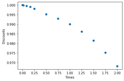
Note that interpolation requires the regression funtion \(f\) at the known points \((x_i, y_i)\) to satisfy \(f(x_i) = y_i\). Therefore, splits points must be \(x_i\), \(i=1,\ldots, n\). Also, note that the default parameter continuous_deriv=True results in spline interpolation.

We generate a time space to calculate interpolated values.

time_space = np.linspace(1/365, 2, 1000)

pw = RobustPWRegression(degree=2, monotonic_trend="descending", solver="ecos")
pw.fit(times, discounts, splits=times)

plt.scatter(times, discounts)
plt.plot(time_space, pw.predict(time_space))

plt.xlabel('Times')
plt.ylabel('Discounts')
plt.show()

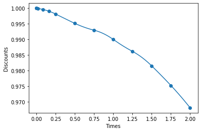
Check interpolated values at split points (known data points).

pw.predict(times)

array([1.       , 0.9999656, 0.9999072, 0.9996074, 0.999004 , 0.9981237,
       0.9951358, 0.9929456, 0.9899849, 0.9861596, 0.9815178, 0.9752363,
       0.9680804])

To interpolate in the rates, it is common to apply a logarithmic transformation on the discount curve. The perform this transformation, set space="log".

pw = RobustPWRegression(degree=3, solver="osqp", space="log")
pw.fit(times, discounts, splits=times)

plt.scatter(times, discounts)
plt.plot(time_space, pw.predict(time_space))

plt.xlabel('Times')
plt.ylabel('Discounts')
plt.show()

Extrapolation

In many applications, we want to extrapolate outside the known points data range. RoPWR introduced extrapolation parameters extrapolation and extrapolation_bounds in version 1.0.0.

Discount curve

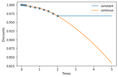
We generate an extended time space. When space="linear" (default) four extrapolation methods are available:

• None: raise exception if value outside \((min(x_i), max(x_i))\)

• “constant”: the value of the regression at \((min(x_i), max(x_i))\) is used for constant extrapolation.

• “continue”: the regression is extrapolated as is.

• “linear”: the regression is linearly extrapolated using the derivatives at \((min(x_i), max(x_i))\).

time_space = np.linspace(0, 5, 1000)

for extrapolation in ("constant", "continue", "linear"):
    pw = RobustPWRegression(degree=3, monotonic_trend="descending", solver="osqp",
                            extrapolation=extrapolation)

    pw.fit(times, discounts, splits=times)

    plt.plot(time_space, pw.predict(time_space), label=f"{extrapolation}")

plt.scatter(times, discounts)

plt.xlabel('Times')
plt.ylabel('Discounts')

plt.legend()
plt.show()

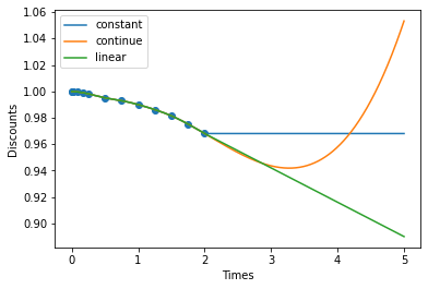
Extrapolation might return unexpected results, especially as the degree increases. For this particular case, we can improve the results using log-space.

for extrapolation in ("constant", "continue"):
    pw = RobustPWRegression(degree=3, monotonic_trend="descending", solver="osqp",
                            extrapolation=extrapolation, space="log")

    pw.fit(times, discounts, splits=times)

    plt.plot(time_space, pw.predict(time_space), label=f"{extrapolation}")

plt.scatter(times, discounts)

plt.xlabel('Times')
plt.ylabel('Discounts')

plt.legend()
plt.show()

Probability default curve

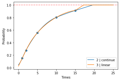
In this section example, we create a probability default curve with 15% deterministic one-year probability of default.

times = np.array([1, 2, 5, 10, 15])
probs = 1 - (1 - 0.15) ** times

time_space = np.linspace(0, 25, 1000)

We set the maximum value to 1 (100% probability) using extrapolation_bounds. If the extrapolated values hit the bounds, constant extrapolation is applied from the intersection points onward.

plt.scatter(times, probs)
plt.axhline(y=1, color='r', linestyle='--', alpha=0.5)

for degree, extrapolation in ((2, "continue"), (3, "linear")):
    pw = RobustPWRegression(degree=degree, monotonic_trend="ascending", solver="osqp",
                            extrapolation=extrapolation, extrapolation_bounds=(0, 1))
    pw.fit(times, probs, splits=times)
    plt.plot(time_space, pw.predict(time_space), label=f'{degree} | {extrapolation}')

plt.xlabel('Times')
plt.ylabel('Probability')

plt.legend()
plt.show()