Tutorial: FICO Explainable Machine Learning Challenge - Updating Binning

In this tutorial, we extend the previous tutorial using the FICO dataset by replacing the usual binning with a piecewise continuous binning. The piecewise continuous binning uses a Gradient Boosting Tree (GBT) as an estimator.

[1]:

import matplotlib.pyplot as plt
import numpy as np
import pandas as pd

[2]:

from lightgbm import LGBMClassifier

from optbinning import BinningProcess
from optbinning import OptimalPWBinning

from sklearn.linear_model import LogisticRegression
from sklearn.ensemble import GradientBoostingClassifier
from sklearn.metrics import classification_report
from sklearn.metrics import auc, roc_auc_score, roc_curve
from sklearn.model_selection import train_test_split

Download the dataset from the link above and load it: https://community.fico.com/s/explainable-machine-learning-challenge.

[3]:

df = pd.read_csv("data/FICO_challenge/heloc_dataset_v1.csv", sep=",")

variable_names = list(df.columns[1:])

X = df[variable_names]

Transform the categorical dichotomic target variable into numerical.

[4]:

y = df.RiskPerformance.values
mask = y == "Bad"
y = mask.astype(int)

Modeling

The data dictionary of this challenge includes three special values/codes:

-9 No Bureau Record or No Investigation
-8 No Usable/Valid Trades or Inquiries
-7 Condition not Met (e.g. No Inquiries, No Delinquencies)

[5]:

special_codes = [-9, -8, -7]

This challenge imposes monotonicity constraints with respect to the probability of a bad target for many of the variables. We apply these rules by passing the following dictionary of parameters for these variables involved.

[6]:

binning_fit_params = {
    "ExternalRiskEstimate": {"monotonic_trend": "descending"},
    "MSinceOldestTradeOpen": {"monotonic_trend": "descending"},
    "MSinceMostRecentTradeOpen": {"monotonic_trend": "descending"},
    "AverageMInFile": {"monotonic_trend": "descending"},
    "NumSatisfactoryTrades": {"monotonic_trend": "descending"},
    "NumTrades60Ever2DerogPubRec": {"monotonic_trend": "ascending"},
    "NumTrades90Ever2DerogPubRec": {"monotonic_trend": "ascending"},
    "PercentTradesNeverDelq": {"monotonic_trend": "descending"},
    "MSinceMostRecentDelq": {"monotonic_trend": "descending"},
    "NumTradesOpeninLast12M": {"monotonic_trend": "ascending"},
    "MSinceMostRecentInqexcl7days": {"monotonic_trend": "descending"},
    "NumInqLast6M": {"monotonic_trend": "ascending"},
    "NumInqLast6Mexcl7days": {"monotonic_trend": "ascending"},
    "NetFractionRevolvingBurden": {"monotonic_trend": "ascending"},
    "NetFractionInstallBurden": {"monotonic_trend": "ascending"},
    "NumBank2NatlTradesWHighUtilization": {"monotonic_trend": "ascending"}
}

Instantiate a BinningProcess object class with variable names, special codes and dictionary of binning parameters. Choose a logistic regression as a classifier.

[7]:

binning_process = BinningProcess(variable_names, special_codes=special_codes,
                                 binning_fit_params=binning_fit_params)

[8]:

clf = LogisticRegression(solver="lbfgs")

Split dataset into train and test. Fit pipelines with training data, then generate classification reports to show the main classification metrics.

[9]:

X_train, X_test, y_train, y_test = train_test_split(X, y, test_size=0.2, random_state=42)

[10]:

binning_process.fit(X_train, y_train)

[10]:

BinningProcess(binning_fit_params={'AverageMInFile': {'monotonic_trend': 'descending'},
                                   'ExternalRiskEstimate': {'monotonic_trend': 'descending'},
                                   'MSinceMostRecentDelq': {'monotonic_trend': 'descending'},
                                   'MSinceMostRecentInqexcl7days': {'monotonic_trend': 'descending'},
                                   'MSinceMostRecentTradeOpen': {'monotonic_trend': 'descending'},
                                   'MSinceOldestTradeOpen': {'mo...
                               'MaxDelq2PublicRecLast12M', 'MaxDelqEver',
                               'NumTotalTrades', 'NumTradesOpeninLast12M',
                               'PercentInstallTrades',
                               'MSinceMostRecentInqexcl7days', 'NumInqLast6M',
                               'NumInqLast6Mexcl7days',
                               'NetFractionRevolvingBurden',
                               'NetFractionInstallBurden',
                               'NumRevolvingTradesWBalance',
                               'NumInstallTradesWBalance',
                               'NumBank2NatlTradesWHighUtilization',
                               'PercentTradesWBalance'])

In a Jupyter environment, please rerun this cell to show the HTML representation or trust the notebook.
On GitHub, the HTML representation is unable to render, please try loading this page with nbviewer.org.

Now, we replace the usual binning of a few numerical variables with a piecewise continuous binning. Since version 0.9.2, the binning process includes the method update_binned_variable which allows updating an optimal binning without the need of re-processing the rest of the variables.

[11]:

update_variables = ["ExternalRiskEstimate", "MSinceOldestTradeOpen", "PercentTradesWBalance"]

for variable in update_variables:
    optb = OptimalPWBinning(estimator=LGBMClassifier(),
                            name=variable, objective="l1")
    optb.fit(X_train[variable], y_train, lb=0.001, ub=0.999)
    binning_process.update_binned_variable(name=variable, optb=optb)

[LightGBM] [Info] Number of positive: 4371, number of negative: 3996
[LightGBM] [Info] Auto-choosing col-wise multi-threading, the overhead of testing was 0.000386 seconds.
You can set `force_col_wise=true` to remove the overhead.
[LightGBM] [Info] Total Bins 54
[LightGBM] [Info] Number of data points in the train set: 8367, number of used features: 1
[LightGBM] [Info] [binary:BoostFromScore]: pavg=0.522409 -> initscore=0.089698
[LightGBM] [Info] Start training from score 0.089698
[LightGBM] [Info] Number of positive: 4371, number of negative: 3996
[LightGBM] [Info] Auto-choosing col-wise multi-threading, the overhead of testing was 0.000342 seconds.
You can set `force_col_wise=true` to remove the overhead.
[LightGBM] [Info] Total Bins 255
[LightGBM] [Info] Number of data points in the train set: 8367, number of used features: 1
[LightGBM] [Info] [binary:BoostFromScore]: pavg=0.522409 -> initscore=0.089698
[LightGBM] [Info] Start training from score 0.089698
[LightGBM] [Info] Number of positive: 4371, number of negative: 3996
[LightGBM] [Info] Auto-choosing col-wise multi-threading, the overhead of testing was 0.000267 seconds.
You can set `force_col_wise=true` to remove the overhead.
[LightGBM] [Info] Total Bins 87
[LightGBM] [Info] Number of data points in the train set: 8367, number of used features: 1
[LightGBM] [Info] [binary:BoostFromScore]: pavg=0.522409 -> initscore=0.089698
[LightGBM] [Info] Start training from score 0.089698

Performance

[12]:

clf.fit(binning_process.transform(X_train), y_train)

[12]:

LogisticRegression()

In a Jupyter environment, please rerun this cell to show the HTML representation or trust the notebook.
On GitHub, the HTML representation is unable to render, please try loading this page with nbviewer.org.

LogisticRegression

?Documentation for LogisticRegressioniFitted

Parameters

	penalty penalty: {'l1', 'l2', 'elasticnet', None}, default='l2' Specify the norm of the penalty: - `None`: no penalty is added; - `'l2'`: add an L2 penalty term and it is the default choice; - `'l1'`: add an L1 penalty term; - `'elasticnet'`: both L1 and L2 penalty terms are added. .. warning:: Some penalties may not work with some solvers. See the parameter `solver` below, to know the compatibility between the penalty and solver. .. versionadded:: 0.19 l1 penalty with SAGA solver (allowing 'multinomial' + L1) .. deprecated:: 1.8 `penalty` was deprecated in version 1.8 and will be removed in 1.10. Use `l1_ratio` and `C` instead. `l1_ratio=0` for `penalty='l2'`, `l1_ratio=1` for `penalty='l1'`, `l1_ratio` set to any float between 0 and 1 for `penalty='elasticnet'`, and `C=np.inf` for `penalty=None`.	'deprecated'
	C C: float, default=1.0 Inverse of regularization strength; must be a positive float. Like in support vector machines, smaller values specify stronger regularization. `C=np.inf` results in unpenalized logistic regression. For a visual example on the effect of tuning the `C` parameter with an L1 penalty, see: :ref:`sphx_glr_auto_examples_linear_model_plot_logistic_path.py`.	1.0
	l1_ratio l1_ratio: float, default=0.0 The Elastic-Net mixing parameter, with `0 <= l1_ratio <= 1`. Setting `l1_ratio=1` gives a pure L1-penalty, setting `l1_ratio=0` a pure L2-penalty. Any value between 0 and 1 gives an Elastic-Net penalty of the form `l1_ratio * L1 + (1 - l1_ratio) * L2`. .. warning:: Certain values of `l1_ratio`, i.e. some penalties, may not work with some solvers. See the parameter `solver` below, to know the compatibility between the penalty and solver. .. versionchanged:: 1.8 Default value changed from None to 0.0. .. deprecated:: 1.8 `None` is deprecated and will be removed in version 1.10. Always use `l1_ratio` to specify the penalty type.	0.0
	dual dual: bool, default=False Dual (constrained) or primal (regularized, see also :ref:`this equation <regularized-logistic-loss>`) formulation. Dual formulation is only implemented for l2 penalty with liblinear solver. Prefer `dual=False` when n_samples > n_features.	False
	tol tol: float, default=1e-4 Tolerance for stopping criteria.	0.0001
	fit_intercept fit_intercept: bool, default=True Specifies if a constant (a.k.a. bias or intercept) should be added to the decision function.	True
	intercept_scaling intercept_scaling: float, default=1 Useful only when the solver `liblinear` is used and `self.fit_intercept` is set to `True`. In this case, `x` becomes `[x, self.intercept_scaling]`, i.e. a "synthetic" feature with constant value equal to `intercept_scaling` is appended to the instance vector. The intercept becomes ``intercept_scaling * synthetic_feature_weight``. .. note:: The synthetic feature weight is subject to L1 or L2 regularization as all other features. To lessen the effect of regularization on synthetic feature weight (and therefore on the intercept) `intercept_scaling` has to be increased.	1
	class_weight class_weight: dict or 'balanced', default=None Weights associated with classes in the form ``{class_label: weight}``. If not given, all classes are supposed to have weight one. The "balanced" mode uses the values of y to automatically adjust weights inversely proportional to class frequencies in the input data as ``n_samples / (n_classes * np.bincount(y))``. Note that these weights will be multiplied with sample_weight (passed through the fit method) if sample_weight is specified. .. versionadded:: 0.17 class_weight='balanced'	None
	random_state random_state: int, RandomState instance, default=None Only used for `solver` == 'sag', 'saga' or 'liblinear' to shuffle the data. It has no effect on the other solvers. See :term:`Glossary <random_state>` for details.	None
	solver solver: {'lbfgs', 'liblinear', 'newton-cg', 'newton-cholesky', 'sag', 'saga'}, default='lbfgs' Algorithm to use in the optimization problem. Default is 'lbfgs'. To choose a solver, you might want to consider the following aspects: - 'lbfgs' is a good default solver because it works reasonably well for a wide class of problems. - For :term:`multiclass` problems (`n_classes >= 3`), all solvers except 'liblinear' minimize the full multinomial loss, 'liblinear' will raise an error. - 'newton-cholesky' is a good choice for `n_samples` >> `n_features * n_classes`, especially with one-hot encoded categorical features with rare categories. Be aware that the memory usage of this solver has a quadratic dependency on `n_features * n_classes` because it explicitly computes the full Hessian matrix. - For small datasets, 'liblinear' is a good choice, whereas 'sag' and 'saga' are faster for large ones; - 'liblinear' can only handle binary classification by default. To apply a one-versus-rest scheme for the multiclass setting one can wrap it with the :class:`~sklearn.multiclass.OneVsRestClassifier`. .. warning:: The choice of the algorithm depends on the penalty chosen (`l1_ratio=0` for L2-penalty, `l1_ratio=1` for L1-penalty and `0 < l1_ratio < 1` for Elastic-Net) and on (multinomial) multiclass support: ================= ======================== ====================== solver l1_ratio multinomial multiclass ================= ======================== ====================== 'lbfgs' l1_ratio=0 yes 'liblinear' l1_ratio=1 or l1_ratio=0 no 'newton-cg' l1_ratio=0 yes 'newton-cholesky' l1_ratio=0 yes 'sag' l1_ratio=0 yes 'saga' 0<=l1_ratio<=1 yes ================= ======================== ====================== .. note:: 'sag' and 'saga' fast convergence is only guaranteed on features with approximately the same scale. You can preprocess the data with a scaler from :mod:`sklearn.preprocessing`. .. seealso:: Refer to the :ref:`User Guide <Logistic_regression>` for more information regarding :class:`LogisticRegression` and more specifically the :ref:`Table <logistic_regression_solvers>` summarizing solver/penalty supports. .. versionadded:: 0.17 Stochastic Average Gradient (SAG) descent solver. Multinomial support in version 0.18. .. versionadded:: 0.19 SAGA solver. .. versionchanged:: 0.22 The default solver changed from 'liblinear' to 'lbfgs' in 0.22. .. versionadded:: 1.2 newton-cholesky solver. Multinomial support in version 1.6.	'lbfgs'
	max_iter max_iter: int, default=100 Maximum number of iterations taken for the solvers to converge.	100
	verbose verbose: int, default=0 For the liblinear and lbfgs solvers set verbose to any positive number for verbosity.	0
	warm_start warm_start: bool, default=False When set to True, reuse the solution of the previous call to fit as initialization, otherwise, just erase the previous solution. Useless for liblinear solver. See :term:`the Glossary <warm_start>`. .. versionadded:: 0.17 warm_start to support lbfgs, newton-cg, sag, saga solvers.	False
	n_jobs n_jobs: int, default=None Does not have any effect. .. deprecated:: 1.8 `n_jobs` is deprecated in version 1.8 and will be removed in 1.10.	None

Fitted attributes

Name	Type	Value
classes_ classes_: ndarray of shape (n_classes, ) A list of class labels known to the classifier.	ndarray[int64](2,)	[0,1]
coef_ coef_: ndarray or CSR matrix of shape (1, n_features) or (n_classes, n_features) Coefficients of the features in the decision function. `coef_` is of shape (1, n_features) when the given problem is binary. By default, it will be created as a dense array, but can be turned to sparse (CSR format) through :meth:`sparsify` (which can be beneficial under L1 regularization when many coefficients are zero), and back to dense through :meth:`densify`.	ndarray[float64](1, 23)	[[-0.16,-0.16,-0.14,..., 0.36,-0.26, 0.07]]
feature_names_in_ feature_names_in_: ndarray of shape (`n_features_in_`,) Names of features seen during :term:`fit`. Defined only when `X` has feature names that are all strings. .. versionadded:: 1.0	ndarray[object](23,)	['ExternalRiskEstimate','MSinceOldestTradeOpen', 'MSinceMostRecentTradeOpen',...,'NumInstallTradesWBalance', 'NumBank2NatlTradesWHighUtilization','PercentTradesWBalance']
intercept_ intercept_: ndarray of shape (1,) or (n_classes,) Intercept (a.k.a. bias) added to the decision function. If `fit_intercept` is set to False, the intercept is set to zero. `intercept_` is of shape (1,) when the given problem is binary.	ndarray[float64](1,)	[0.]
n_features_in_ n_features_in_: int Number of features seen during :term:`fit`. .. versionadded:: 0.24	int	23
n_iter_ n_iter_: ndarray of shape (1, ) Actual number of iterations for all classes. .. versionchanged:: 0.20 In SciPy <= 1.0.0 the number of lbfgs iterations may exceed ``max_iter``. ``n_iter_`` will now report at most ``max_iter``.	ndarray[int32](1,)	[35]

[13]:

y_pred = clf.predict(binning_process.transform(X_test))
print(classification_report(y_test, y_pred))

              precision    recall  f1-score   support

           0       0.71      0.67      0.69      1004
           1       0.71      0.74      0.72      1088

    accuracy                           0.71      2092
   macro avg       0.71      0.71      0.71      2092
weighted avg       0.71      0.71      0.71      2092

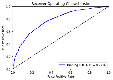
If we compare with the results from the previous tutorial, we observe a slight improvement in all three metrics.

[14]:

probs = clf.predict_proba(binning_process.transform(X_test))
preds = probs[:,1]
fpr1, tpr1, threshold = roc_curve(y_test, preds)
roc_auc1 = auc(fpr1, tpr1)

[15]:

plt.title('Receiver Operating Characteristic')
plt.plot(fpr1, tpr1, 'b', label='Binning+LR: AUC = {0:.4f}'.format(roc_auc1))
plt.legend(loc='lower right')
plt.plot([0, 1], [0, 1],'k--')
plt.xlim([0, 1])
plt.ylim([0, 1])
plt.ylabel('True Positive Rate')
plt.xlabel('False Positive Rate')
plt.show()

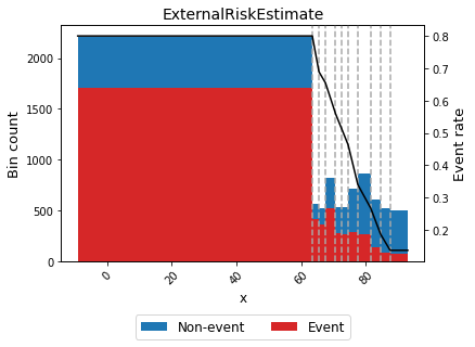
../_images/tutorials_tutorial_binning_process_FICO_update_binning_26_0.png

Finally, let’s check the piecewise continuous binning for one of the variables with more importance.

[16]:

optb = binning_process.get_binned_variable("ExternalRiskEstimate")
optb.binning_table.build()

[16]:

	Bin	Count	Count (%)	Non-event	Event	c0	c1
0	(-inf, 63.50)	2213	0.264491	510	1703	0.799992	0.0
1	[63.50, 65.50)	563	0.067288	153	410	4.297018	-0.055071
2	[65.50, 67.50)	516	0.061671	157	359	1.785794	-0.016732
3	[67.50, 70.50)	824	0.098482	307	517	2.741961	-0.030897
4	[70.50, 72.50)	530	0.063344	258	272	2.295718	-0.024568
5	[72.50, 74.50)	530	0.063344	265	265	2.285798	-0.024431
6	[74.50, 77.50)	709	0.084738	423	286	3.568892	-0.041654
7	[77.50, 81.50)	864	0.103263	600	264	1.746826	-0.018143
8	[81.50, 84.50)	602	0.071949	461	141	2.45228	-0.026799
9	[84.50, 87.50)	518	0.061910	437	81	1.635314	-0.017131
10	[87.50, inf)	498	0.059520	425	73	0.136374	0.0
11	Special	0	0.000000	0	0	0.0	0.0
12	Missing	0	0.000000	0	0	0.0	0.0
Totals		8367	1.000000	3996	4371	-	-

[17]:

optb.binning_table.analysis()

---------------------------------------------
OptimalBinning: Binary Binning Table Analysis
---------------------------------------------

  General metrics

    Gini index               0.51846722
    IV (Jeffrey)             1.02947556
    JS (Jensen-Shannon)      0.11880538
    Hellinger                0.12345589
    Triangular               0.44355285
    KS                       0.40393001
    Avg precision            0.73645607
    Brier score              0.19906995
    HHI                      0.12640619
    HHI (normalized)         0.03904681
    Cramer's V               0.45085066
    Quality score            0.01120736

  Significance tests

    Bin A  Bin B  t-statistic  p-value  P[A > B]  P[B > A]
        0      1     4.273551 0.038710  0.979402  0.020598
        1      2     1.388516 0.238656  0.880875  0.119125
        2      3     6.506519 0.010748  0.995084  0.004916
        3      4    17.292596 0.000032  0.999996  0.000004
        4      5     0.184590 0.667458  0.666430  0.333570
        5      6    11.450667 0.000715  0.999713  0.000287
        6      7    16.377781 0.000052  0.999986  0.000014
        7      8     8.982480 0.002726  0.999028  0.000972
        8      9    10.554598 0.001159  0.999629  0.000371
        9     10     0.186908 0.665503  0.667979  0.332021

[18]:

optb.binning_table.plot(metric="event_rate")

../_images/tutorials_tutorial_binning_process_FICO_update_binning_30_0.png

[19]:

binning_process.summary()

[19]:

	name	dtype	status	selected	n_bins	iv	js	gini	quality_score
0	ExternalRiskEstimate	numerical	OPTIMAL	True	11	1.029476	0.118805	0.518467	0.011207
1	MSinceOldestTradeOpen	numerical	OPTIMAL	True	10	0.226679	0.027774	0.256181	0.014071
2	MSinceMostRecentTradeOpen	numerical	OPTIMAL	True	6	0.019086	0.002377	0.065597	0.000567
3	AverageMInFile	numerical	OPTIMAL	True	10	0.319379	0.038458	0.304157	0.129149
4	NumSatisfactoryTrades	numerical	OPTIMAL	True	10	0.126726	0.015424	0.180888	0.00122
5	NumTrades60Ever2DerogPubRec	numerical	OPTIMAL	True	4	0.17871	0.021915	0.200184	0.210032
6	NumTrades90Ever2DerogPubRec	numerical	OPTIMAL	True	3	0.133485	0.016301	0.155193	0.305629
7	PercentTradesNeverDelq	numerical	OPTIMAL	True	8	0.377803	0.045428	0.316946	0.102689
8	MSinceMostRecentDelq	numerical	OPTIMAL	True	7	0.289526	0.035246	0.272229	0.243295
9	MaxDelq2PublicRecLast12M	numerical	OPTIMAL	True	3	0.33028	0.04025	0.30167	0.889293
10	MaxDelqEver	numerical	OPTIMAL	True	4	0.236098	0.029129	0.257314	0.695771
11	NumTotalTrades	numerical	OPTIMAL	True	8	0.064716	0.008027	0.138545	0.011902
12	NumTradesOpeninLast12M	numerical	OPTIMAL	True	6	0.02353	0.002936	0.08377	0.008097
13	PercentInstallTrades	numerical	OPTIMAL	True	8	0.09861	0.012107	0.159569	0.078373
14	MSinceMostRecentInqexcl7days	numerical	OPTIMAL	True	4	0.166538	0.02046	0.211639	0.553168
15	NumInqLast6M	numerical	OPTIMAL	True	4	0.089956	0.011127	0.159369	0.337271
16	NumInqLast6Mexcl7days	numerical	OPTIMAL	True	5	0.083992	0.010394	0.153641	0.037328
17	NetFractionRevolvingBurden	numerical	OPTIMAL	True	9	0.574686	0.068232	0.410605	0.347064
18	NetFractionInstallBurden	numerical	OPTIMAL	True	5	0.037879	0.004724	0.105916	0.055258
19	NumRevolvingTradesWBalance	numerical	OPTIMAL	True	7	0.093376	0.011578	0.162108	0.01147
20	NumInstallTradesWBalance	numerical	OPTIMAL	True	5	0.014121	0.001762	0.059437	0.010721
21	NumBank2NatlTradesWHighUtilization	numerical	OPTIMAL	True	5	0.334853	0.041017	0.308402	0.228472
22	PercentTradesWBalance	numerical	OPTIMAL	True	13	0.379238	0.04583	0.333975	0.018462