Tutorial: FICO Explainable Machine Learning Challenge
In this tutorial, we use the dataset form the FICO Explainable Machine Learning Challenge: https://community.fico.com/s/explainable-machine-learning-challenge. The goal is to create a pipeline by combining a binning process and logistic regression to obtain an explainable model and compare it against a black-box model using Gradient Boosting Tree (GBT) as an estimator.
[1]:
import matplotlib.pyplot as plt
import numpy as np
import pandas as pd
[2]:
from optbinning import BinningProcess

from sklearn.linear_model import LogisticRegression
from sklearn.ensemble import GradientBoostingClassifier
from sklearn.metrics import classification_report
from sklearn.metrics import auc, roc_auc_score, roc_curve
from sklearn.model_selection import train_test_split
from sklearn.pipeline import Pipeline
Download the dataset from the link above and load it.
[3]:
df = pd.read_csv("data/FICO_challenge/heloc_dataset_v1.csv", sep=",")
[4]:
variable_names = list(df.columns[1:])
[5]:
X = df[variable_names].values
Transform the categorical dichotomic target variable into numerical.
[6]:
y = df.RiskPerformance.values
mask = y == "Bad"
y[mask] = 1
y[~mask] = 0
y = y.astype(int)
Modeling
The data dictionary of this challenge includes three special values/codes:
-9 No Bureau Record or No Investigation
-8 No Usable/Valid Trades or Inquiries
-7 Condition not Met (e.g. No Inquiries, No Delinquencies)
[7]:
special_codes = [-9, -8, -7]
This challenge imposes monotonicity constraints with respect to the probability of a bad target for many of the variables. We apply these rules by passing the following dictionary of parameters for these variables involved.
[8]:
binning_fit_params = {
    "ExternalRiskEstimate": {"monotonic_trend": "descending"},
    "MSinceOldestTradeOpen": {"monotonic_trend": "descending"},
    "MSinceMostRecentTradeOpen": {"monotonic_trend": "descending"},
    "AverageMInFile": {"monotonic_trend": "descending"},
    "NumSatisfactoryTrades": {"monotonic_trend": "descending"},
    "NumTrades60Ever2DerogPubRec": {"monotonic_trend": "ascending"},
    "NumTrades90Ever2DerogPubRec": {"monotonic_trend": "ascending"},
    "PercentTradesNeverDelq": {"monotonic_trend": "descending"},
    "MSinceMostRecentDelq": {"monotonic_trend": "descending"},
    "NumTradesOpeninLast12M": {"monotonic_trend": "ascending"},
    "MSinceMostRecentInqexcl7days": {"monotonic_trend": "descending"},
    "NumInqLast6M": {"monotonic_trend": "ascending"},
    "NumInqLast6Mexcl7days": {"monotonic_trend": "ascending"},
    "NetFractionRevolvingBurden": {"monotonic_trend": "ascending"},
    "NetFractionInstallBurden": {"monotonic_trend": "ascending"},
    "NumBank2NatlTradesWHighUtilization": {"monotonic_trend": "ascending"}
}
Instantiate a BinningProcess object class with variable names, special codes and dictionary of binning parameters. Create a explainable model pipeline and a black-blox pipeline.
[9]:
binning_process = BinningProcess(variable_names, special_codes=special_codes,
                                 binning_fit_params=binning_fit_params)
[10]:
clf1 = Pipeline(steps=[('binning_process', binning_process),
                      ('classifier', LogisticRegression(solver="lbfgs"))])

clf2 = LogisticRegression(solver="lbfgs")

clf3 = GradientBoostingClassifier()
Split dataset into train and test. Fit pipelines with training data, then generate classification reports to show the main classification metrics.
[11]:
X_train, X_test, y_train, y_test = train_test_split(X, y, test_size=0.2, random_state=42)
[12]:
clf1.fit(X_train, y_train)
/home/gui/projects/github/top/optbinning/optbinning/binning/transformations.py:38: RuntimeWarning: invalid value encountered in log
  return np.log((1. / event_rate - 1) * n_event / n_nonevent)
[12]:
Pipeline(steps=[('binning_process',
                 BinningProcess(binning_fit_params={'AverageMInFile': {'monotonic_trend': 'descending'},
                                                    'ExternalRiskEstimate': {'monotonic_trend': 'descending'},
                                                    'MSinceMostRecentDelq': {'monotonic_trend': 'descending'},
                                                    'MSinceMostRecentInqexcl7days': {'monotonic_trend': 'descending'},
                                                    'MSinceMostRecentTradeOpen': {'monotonic_trend': 'descen...
                                                'MaxDelqEver', 'NumTotalTrades',
                                                'NumTradesOpeninLast12M',
                                                'PercentInstallTrades',
                                                'MSinceMostRecentInqexcl7days',
                                                'NumInqLast6M',
                                                'NumInqLast6Mexcl7days',
                                                'NetFractionRevolvingBurden',
                                                'NetFractionInstallBurden',
                                                'NumRevolvingTradesWBalance',
                                                'NumInstallTradesWBalance',
                                                'NumBank2NatlTradesWHighUtilization',
                                                'PercentTradesWBalance'])),
                ('classifier', LogisticRegression())])
[13]:
clf2.fit(X_train, y_train)
/home/gui/anaconda3/lib/python3.7/site-packages/sklearn/linear_model/_logistic.py:818: ConvergenceWarning: lbfgs failed to converge (status=1):
STOP: TOTAL NO. of ITERATIONS REACHED LIMIT.

Increase the number of iterations (max_iter) or scale the data as shown in:
    https://scikit-learn.org/stable/modules/preprocessing.html
Please also refer to the documentation for alternative solver options:
    https://scikit-learn.org/stable/modules/linear_model.html#logistic-regression
  extra_warning_msg=_LOGISTIC_SOLVER_CONVERGENCE_MSG,
[13]:
LogisticRegression()
[14]:
clf3.fit(X_train, y_train)
[14]:
GradientBoostingClassifier()
[15]:
y_pred = clf1.predict(X_test)
print(classification_report(y_test, y_pred))
              precision    recall  f1-score   support

           0       0.70      0.66      0.68      1004
           1       0.70      0.74      0.72      1088

    accuracy                           0.70      2092
   macro avg       0.70      0.70      0.70      2092
weighted avg       0.70      0.70      0.70      2092
/home/gui/projects/github/top/optbinning/optbinning/binning/transformations.py:38: RuntimeWarning: invalid value encountered in log
  return np.log((1. / event_rate - 1) * n_event / n_nonevent)
[16]:
y_pred = clf2.predict(X_test)
print(classification_report(y_test, y_pred))
              precision    recall  f1-score   support

           0       0.67      0.66      0.67      1004
           1       0.69      0.70      0.70      1088

    accuracy                           0.68      2092
   macro avg       0.68      0.68      0.68      2092
weighted avg       0.68      0.68      0.68      2092
[17]:
y_pred = clf3.predict(X_test)
print(classification_report(y_test, y_pred))
              precision    recall  f1-score   support

           0       0.71      0.66      0.68      1004
           1       0.70      0.75      0.73      1088

    accuracy                           0.71      2092
   macro avg       0.71      0.70      0.70      2092
weighted avg       0.71      0.71      0.70      2092
Plot the Receiver Operating Characteristic (ROC) metric to evaluate and compare the classifiers’ prediction.
[18]:
probs = clf1.predict_proba(X_test)
preds = probs[:,1]
fpr1, tpr1, threshold = roc_curve(y_test, preds)
roc_auc1 = auc(fpr1, tpr1)

probs = clf2.predict_proba(X_test)
preds = probs[:,1]
fpr2, tpr2, threshold = roc_curve(y_test, preds)
roc_auc2 = auc(fpr2, tpr2)

probs = clf3.predict_proba(X_test)
preds = probs[:,1]
fpr3, tpr3, threshold = roc_curve(y_test, preds)
roc_auc3 = auc(fpr3, tpr3)
/home/gui/projects/github/top/optbinning/optbinning/binning/transformations.py:38: RuntimeWarning: invalid value encountered in log
  return np.log((1. / event_rate - 1) * n_event / n_nonevent)
[19]:
plt.title('Receiver Operating Characteristic')
plt.plot(fpr1, tpr1, 'b', label='Binning+LR: AUC = {0:.2f}'.format(roc_auc1))
plt.plot(fpr2, tpr2, 'g', label='LR: AUC = {0:.2f}'.format(roc_auc2))
plt.plot(fpr3, tpr3, 'r', label='GBT: AUC = {0:.2f}'.format(roc_auc3))
plt.legend(loc='lower right')
plt.plot([0, 1], [0, 1],'k--')
plt.xlim([0, 1])
plt.ylim([0, 1])
plt.ylabel('True Positive Rate')
plt.xlabel('False Positive Rate')
plt.show()
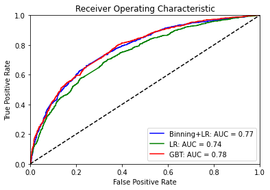
The plot above shows the increment in terms of model performance after binning when the logistic estimator is chosen. Furthermore, a previous binning process might reduce numerical instability issues, as confirmed when fitting the classifier clf2.
Binning process statistics
The binning process of the pipeline can be retrieved to show information about the problem and timing statistics.
[20]:
binning_process.information(print_level=2)
optbinning (Version 0.19.0)
Copyright (c) 2019-2024 Guillermo Navas-Palencia, Apache License 2.0

  Begin options
    max_n_prebins                         20   * d
    min_prebin_size                     0.05   * d
    min_n_bins                            no   * d
    max_n_bins                            no   * d
    min_bin_size                          no   * d
    max_bin_size                          no   * d
    max_pvalue                            no   * d
    max_pvalue_policy            consecutive   * d
    selection_criteria                    no   * d
    fixed_variables                       no   * d
    categorical_variables                 no   * d
    special_codes                        yes   * U
    split_digits                          no   * d
    binning_fit_params                   yes   * U
    binning_transform_params              no   * d
    verbose                            False   * d
  End options

  Statistics
    Number of records                   8367
    Number of variables                   23
    Target type                       binary

    Number of numerical                   23
    Number of categorical                  0
    Number of selected                    23

  Time                                2.3069 sec
The summary method returns basic statistics for each binned variable.
[21]:
binning_process.summary()
[21]:
| name | dtype | status | selected | n_bins | iv | js | gini | quality_score | |
|---|---|---|---|---|---|---|---|---|---|
| 0 | ExternalRiskEstimate | numerical | OPTIMAL | True | 12 | 1.018368 | 0.116638 | 0.534387 | 0.031792 |
| 1 | MSinceOldestTradeOpen | numerical | OPTIMAL | True | 11 | 0.252786 | 0.030483 | 0.264740 | 0.027179 |
| 2 | MSinceMostRecentTradeOpen | numerical | OPTIMAL | True | 6 | 0.019086 | 0.002377 | 0.065597 | 0.000556 |
| 3 | AverageMInFile | numerical | OPTIMAL | True | 10 | 0.319379 | 0.038458 | 0.304157 | 0.128082 |
| 4 | NumSatisfactoryTrades | numerical | OPTIMAL | True | 10 | 0.126726 | 0.015424 | 0.180888 | 0.001210 |
| 5 | NumTrades60Ever2DerogPubRec | numerical | OPTIMAL | True | 4 | 0.178710 | 0.021915 | 0.200184 | 0.201631 |
| 6 | NumTrades90Ever2DerogPubRec | numerical | OPTIMAL | True | 3 | 0.133485 | 0.016301 | 0.155193 | 0.286527 |
| 7 | PercentTradesNeverDelq | numerical | OPTIMAL | True | 8 | 0.377803 | 0.045428 | 0.316946 | 0.101421 |
| 8 | MSinceMostRecentDelq | numerical | OPTIMAL | True | 7 | 0.289526 | 0.035246 | 0.272229 | 0.239494 |
| 9 | MaxDelq2PublicRecLast12M | numerical | OPTIMAL | True | 3 | 0.330280 | 0.040250 | 0.301670 | 0.833712 |
| 10 | MaxDelqEver | numerical | OPTIMAL | True | 4 | 0.236098 | 0.029129 | 0.257314 | 0.667940 |
| 11 | NumTotalTrades | numerical | OPTIMAL | True | 8 | 0.064716 | 0.008027 | 0.138545 | 0.011755 |
| 12 | NumTradesOpeninLast12M | numerical | OPTIMAL | True | 6 | 0.023530 | 0.002936 | 0.083770 | 0.007932 |
| 13 | PercentInstallTrades | numerical | OPTIMAL | True | 8 | 0.098610 | 0.012107 | 0.159569 | 0.077405 |
| 14 | MSinceMostRecentInqexcl7days | numerical | OPTIMAL | True | 4 | 0.166538 | 0.020460 | 0.211639 | 0.531041 |
| 15 | NumInqLast6M | numerical | OPTIMAL | True | 4 | 0.089956 | 0.011127 | 0.159369 | 0.323780 |
| 16 | NumInqLast6Mexcl7days | numerical | OPTIMAL | True | 5 | 0.083992 | 0.010394 | 0.153641 | 0.036291 |
| 17 | NetFractionRevolvingBurden | numerical | OPTIMAL | True | 9 | 0.574686 | 0.068232 | 0.410605 | 0.343593 |
| 18 | NetFractionInstallBurden | numerical | OPTIMAL | True | 5 | 0.037879 | 0.004724 | 0.105916 | 0.053723 |
| 19 | NumRevolvingTradesWBalance | numerical | OPTIMAL | True | 7 | 0.093376 | 0.011578 | 0.162108 | 0.011291 |
| 20 | NumInstallTradesWBalance | numerical | OPTIMAL | True | 5 | 0.014121 | 0.001762 | 0.059437 | 0.010423 |
| 21 | NumBank2NatlTradesWHighUtilization | numerical | OPTIMAL | True | 5 | 0.334853 | 0.041017 | 0.308402 | 0.222126 |
| 22 | PercentTradesWBalance | numerical | OPTIMAL | True | 12 | 0.365412 | 0.044210 | 0.334112 | 0.018131 |
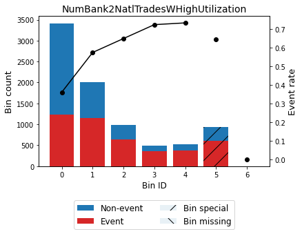
The get_binned_variable method serves to retrieve an optimal binning object, which can be analyzed in detail afterward.
[22]:
optb = binning_process.get_binned_variable("NumBank2NatlTradesWHighUtilization")
[23]:
optb.binning_table.build()
[23]:
| Bin | Count | Count (%) | Non-event | Event | Event rate | WoE | IV | JS | |
|---|---|---|---|---|---|---|---|---|---|
| 0 | (-inf, 0.50) | 3416 | 0.408271 | 2184 | 1232 | 0.360656 | 0.662217 | 0.175281 | 0.021518 |
| 1 | [0.50, 1.50) | 2015 | 0.240827 | 858 | 1157 | 0.574194 | -0.209284 | 0.010461 | 0.001305 |
| 2 | [1.50, 2.50) | 983 | 0.117485 | 345 | 638 | 0.649034 | -0.525096 | 0.031309 | 0.003869 |
| 3 | [2.50, 3.50) | 496 | 0.059281 | 137 | 359 | 0.723790 | -0.873644 | 0.041802 | 0.005065 |
| 4 | [3.50, inf) | 521 | 0.062268 | 139 | 382 | 0.733205 | -0.921249 | 0.048466 | 0.005853 |
| 5 | Special | 936 | 0.111868 | 333 | 603 | 0.644231 | -0.504077 | 0.027533 | 0.003406 |
| 6 | Missing | 0 | 0.000000 | 0 | 0 | 0.000000 | 0.000000 | 0.000000 | 0.000000 |
| Totals | 8367 | 1.000000 | 3996 | 4371 | 0.522409 | 0.334853 | 0.041017 |
[24]:
optb.binning_table.plot(metric="event_rate")
[25]:
optb.binning_table.analysis()
---------------------------------------------
OptimalBinning: Binary Binning Table Analysis
---------------------------------------------

  General metrics

    Gini index               0.30840174
    IV (Jeffrey)             0.33485338
    JS (Jensen-Shannon)      0.04101657
    Hellinger                0.04143062
    Triangular               0.16088993
    KS                       0.26468885
    HHI                      0.25839135
    HHI (normalized)         0.13478991
    Cramer's V               0.28612357
    Quality score            0.22212566

  Monotonic trend             ascending

  Significance tests

    Bin A  Bin B  t-statistic      p-value      P[A > B]  P[B > A]
        0      1   234.556206 6.049946e-53 5.576352e-107  1.000000
        1      2    15.402738 8.686234e-05  7.665294e-06  0.999992
        2      3     8.386138 3.780934e-03  1.290940e-03  0.998709
        3      4     0.113909 7.357368e-01  3.678894e-01  0.632111