Tutorial: optimal piecewise binning with binary target

Basic

To get us started, let’s load a well-known dataset from the UCI repository and transform the data into a pandas.DataFrame.

[1]:

import numpy as np
import pandas as pd

from sklearn.datasets import load_breast_cancer
from sklearn.ensemble import GradientBoostingClassifier

[2]:

data = load_breast_cancer()
df = pd.DataFrame(data.data, columns=data.feature_names)

We choose a variable to discretize and the binary target.

[3]:

variable = "mean radius"
x = df[variable].values
y = data.target

Import and instantiate an OptimalPWBinning object class and we pass the variable name. The OptimalPWBinning can ONLY handle numerical variables. This differs from the OptimalBinning object class.

[4]:

from optbinning import OptimalPWBinning

[5]:

optb = OptimalPWBinning(name=variable)

We fit the optimal binning object with arrays x and y. We set a minimum (lower bound) and maximum (upper bound) probability using arguments lb and ub. Note that these bounds are optional, but guarantee an event rate between \([0, 1]\) as any probability distribution. As shown later, settings these bounds will increase the problem size thus leading to higher solution times. An alternative approach to bypass these bounds is implemented when transforming to event rate or WoE using functions fit and fit_transform, where values outside the interval \([0, 1]\) are clipped.

Note that the Weight-of-Evidence is not defined for event rate equal 0 or 1. Therefore, for small datasets, we recommend modifying the interval \([0, 1]\) with a small value, thus using \([\epsilon, 1 - \epsilon]\).

[6]:

optb.fit(x, y, lb=0.001, ub=0.999)

[6]:

OptimalPWBinning(estimator=LogisticRegression(), name='mean radius')

In a Jupyter environment, please rerun this cell to show the HTML representation or trust the notebook.
On GitHub, the HTML representation is unable to render, please try loading this page with nbviewer.org.

You can check if an optimal solution has been found via the status attribute:

[7]:

optb.status

[7]:

'OPTIMAL'

You can also retrieve the optimal split points via the splits attribute:

[8]:

optb.splits

[8]:

array([11.42500019, 12.32999992, 13.09499979, 13.70499992, 15.04500008,
       16.92500019])

The binning table

The optimal binning algorithms return a binning table; a binning table displays the binned data and several metrics for each bin. Class OptimalPWBinning returns an object PWBinningTable via the binning_table attribute.

[9]:

binning_table = optb.binning_table

[10]:

type(binning_table)

[10]:

optbinning.binning.piecewise.binning_statistics.PWBinningTable

The binning_table is instantiated, but not built. Therefore, the first step is to call the method build, which returns a pandas.DataFrame.

[11]:

binning_table.build()

[11]:

	Bin	Count	Count (%)	Non-event	Event	c0	c1
0	(-inf, 11.43)	118	0.207381	3	115	1.032597	-0.004813
1	[11.43, 12.33)	79	0.138840	3	76	1.644465	-0.058368
2	[12.33, 13.09)	68	0.119508	7	61	2.140581	-0.098604
3	[13.09, 13.70)	49	0.086116	10	39	2.915209	-0.157759
4	[13.70, 15.05)	83	0.145870	28	55	4.107004	-0.244719
5	[15.05, 16.93)	54	0.094903	44	10	3.562027	-0.208496
6	[16.93, inf)	118	0.207381	117	1	0.081993	-0.002881
7	Special	0	0.000000	0	0	0.0	0.0
8	Missing	0	0.000000	0	0	0.0	0.0
Totals		569	1.000000	212	357	-	-

Let’s describe the columns of this binning table:

Bin: the intervals delimited by the optimal split points.
Count: the number of records for each bin.
Count (%): the percentage of records for each bin.
Non-event: the number of non-event records \((y = 0)\) for each bin.
Event: the number of event records \((y = 1)\) for each bin.
\(c_0\): the first coefficient of the event rate polynomial.
\(c_1\): the second coefficient of the event rate polynomial.

The event rate for bin \(i\) is defined as \(ER_i = c_0 + c_1 x_i\), where \(x_i \in \text{Bin}_{i}\). In general, \begin{equation} ER_i = \sum_{j=0}^d c_j x_i^j, \end{equation} where \(d\) is the degree of the event rate polynomial.

The last row shows the total number of records, non-event records, event records.

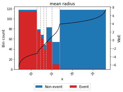
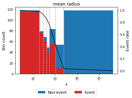
You can use the method plot to visualize the number of non-event and event records by bin, and WoE or event rate curve.

[12]:

binning_table.plot(metric="woe")

../_images/tutorials_tutorial_piecewise_binary_24_0.png

[13]:

binning_table.plot(metric="event_rate")

../_images/tutorials_tutorial_piecewise_binary_25_0.png

Event rate / WoE transformation

Now that we have checked the binned data, we can transform our original data into WoE or event rate values.

[14]:

x_transform_woe = optb.transform(x, metric="woe")

[15]:

x_transform_event_rate = optb.transform(x, metric="event_rate")

Advanced

Optimal binning Information

The OptimalPWBinning can print overview information about the options settings, problem statistics, and the solution of the computation. By default, print_level=1.

[16]:

optb = OptimalPWBinning(name=variable)
optb.fit(x, y)

[16]:

OptimalPWBinning(estimator=LogisticRegression(), name='mean radius')

In a Jupyter environment, please rerun this cell to show the HTML representation or trust the notebook.
On GitHub, the HTML representation is unable to render, please try loading this page with nbviewer.org.

If print_level=0, a minimal output including the header, variable name, status, and total time are printed.

[17]:

optb.information(print_level=0)

optbinning (Version 1.0.0)
Copyright (c) 2019-2026 Guillermo Navas-Palencia, Apache License 2.0

  Name    : mean radius
  Status  : OPTIMAL

  Time    : 0.5454  sec

If print_level>=1, statistics on the pre-binning phase and the solver are printed. More detailed timing statistics are also included.

[18]:

optb.information(print_level=1)

optbinning (Version 1.0.0)
Copyright (c) 2019-2026 Guillermo Navas-Palencia, Apache License 2.0

  Name    : mean radius
  Status  : OPTIMAL

  Pre-binning statistics
    Number of bins                         7

  Solver statistics
    Type                                auto
    Number of variables                   14
    Number of constraints                 20

  Timing
    Total time                          0.55 sec
    Pre-processing                      0.00 sec   (  0.06%)
    Estimator                           0.15 sec   ( 26.87%)
    Pre-binning                         0.21 sec   ( 38.29%)
    Solver                              0.16 sec   ( 30.09%)
    Post-processing                     0.02 sec   (  4.49%)

If print_level=2, the list of all options of the OptimalBinning are displayed.

[19]:

optb.information(print_level=2)

optbinning (Version 1.0.0)
Copyright (c) 2019-2026 Guillermo Navas-Palencia, Apache License 2.0

  Begin options
    name                         mean radius   * U
    estimator                            yes   * U
    objective                             l2   * d
    degree                                 1   * d
    continuous                          True   * d
    prebinning_method                   cart   * d
    max_n_prebins                         20   * d
    min_prebin_size                     0.05   * d
    min_n_bins                            no   * d
    max_n_bins                            no   * d
    min_bin_size                          no   * d
    max_bin_size                          no   * d
    monotonic_trend                     auto   * d
    n_subsamples                          no   * d
    max_pvalue                            no   * d
    max_pvalue_policy            consecutive   * d
    outlier_detector                      no   * d
    outlier_params                        no   * d
    user_splits                           no   * d
    special_codes                         no   * d
    split_digits                          no   * d
    solver                              auto   * d
    h_epsilon                           1.35   * d
    quantile                             0.5   * d
    regularization                        no   * d
    reg_l1                               1.0   * d
    reg_l2                               1.0   * d
    random_state                          no   * d
    verbose                            False   * d
  End options

  Name    : mean radius
  Status  : OPTIMAL

  Pre-binning statistics
    Number of bins                         7

  Solver statistics
    Type                                auto
    Number of variables                   14
    Number of constraints                 20

  Timing
    Total time                          0.55 sec
    Pre-processing                      0.00 sec   (  0.06%)
    Estimator                           0.15 sec   ( 26.87%)
    Pre-binning                         0.21 sec   ( 38.29%)
    Solver                              0.16 sec   ( 30.09%)
    Post-processing                     0.02 sec   (  4.49%)

Binning table statistical analysis

The analysis method performs a statistical analysis of the binning table, computing the statistics Gini index, Information Value (IV), Jensen-Shannon divergence, and the quality score. Additionally, several statistical significance tests between consecutive bins of the contingency table are performed: a frequentist test using the Chi-square test or the Fisher’s exact test, and a Bayesian A/B test using the beta distribution as a conjugate prior of the Bernoulli distribution. The piecewise binning also includes two performance metrics: the average precision and the Brier score.

[20]:

binning_table.analysis(pvalue_test="chi2")

---------------------------------------------
OptimalBinning: Binary Binning Table Analysis
---------------------------------------------

  General metrics

    Gini index               0.87503303
    IV (Jeffrey)             4.48034999
    JS (Jensen-Shannon)      0.37576960
    Hellinger                0.44284048
    Triangular               1.20890940
    KS                       0.72390466
    Avg precision            0.95577179
    Brier score              0.08956359
    HHI                      0.15727342
    HHI (normalized)         0.01681899
    Cramer's V               0.80066760
    Quality score            0.00000000

  Significance tests

    Bin A  Bin B  t-statistic      p-value  P[A > B]     P[B > A]
        0      1     0.289789 5.903557e-01  0.697563 3.024368e-01
        1      2     2.285355 1.306002e-01  0.941469 5.853092e-02
        2      3     2.317546 1.279217e-01  0.936661 6.333919e-02
        3      4     2.539025 1.110634e-01  0.950869 4.913141e-02
        4      5    29.418844 5.830790e-08  1.000000 1.898159e-11
        5      6    18.624518 1.591604e-05  0.999997 3.106835e-06

[21]:

binning_table.analysis(pvalue_test="fisher")

---------------------------------------------
OptimalBinning: Binary Binning Table Analysis
---------------------------------------------

  General metrics

    Gini index               0.87503303
    IV (Jeffrey)             4.48034999
    JS (Jensen-Shannon)      0.37576960
    Hellinger                0.44284048
    Triangular               1.20890940
    KS                       0.72390466
    Avg precision            0.95577179
    Brier score              0.08956359
    HHI                      0.15727342
    HHI (normalized)         0.01681899
    Cramer's V               0.80066760
    Quality score            0.00000000

  Significance tests

    Bin A  Bin B  odd ratio      p-value  P[A > B]     P[B > A]
        0      1   0.660870 6.855009e-01  0.697563 3.024368e-01
        1      2   0.343985 1.879769e-01  0.941469 5.853092e-02
        2      3   0.447541 1.829850e-01  0.936661 6.333919e-02
        3      4   0.503663 1.153088e-01  0.950869 4.913141e-02
        4      5   0.115702 3.464724e-08  1.000000 1.898148e-11
        5      6   0.037607 4.144258e-05  0.999997 3.106835e-06

Event rate / WoE monotonicity

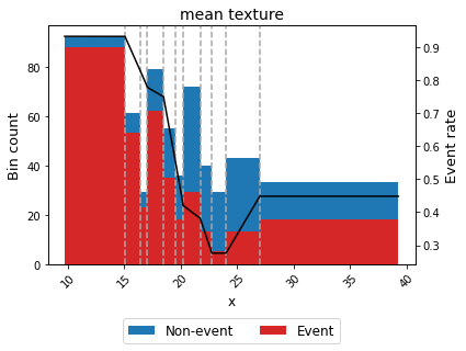
The monotonic_trend option permits forcing a monotonic trend to the event rate curve. The default setting “auto” should be the preferred option, however, some business constraints might require to impose different trends. The default setting “auto” chooses the monotonic trend most likely to maximize the information value from the options “ascending”, “descending”, “peak” and “valley” using a machine-learning-based classifier. For this example, we choose Gradient Boosting as an estimator.

[22]:

variable = "mean texture"
x = df[variable].values
y = data.target

[23]:

optb = OptimalPWBinning(name=variable, estimator=GradientBoostingClassifier())
optb.fit(x, y, lb=0.001, ub=0.999)

[23]:

OptimalPWBinning(estimator=GradientBoostingClassifier(), name='mean texture')

In a Jupyter environment, please rerun this cell to show the HTML representation or trust the notebook.
On GitHub, the HTML representation is unable to render, please try loading this page with nbviewer.org.

[24]:

binning_table = optb.binning_table
binning_table.build()

[24]:

	Bin	Count	Count (%)	Non-event	Event	c0	c1
0	(-inf, 15.05)	92	0.161687	4	88	0.931559	-0.0
1	[15.05, 16.39)	61	0.107206	8	53	2.075855	-0.076058
2	[16.39, 17.03)	29	0.050967	6	23	2.149387	-0.080543
3	[17.03, 18.46)	79	0.138840	17	62	1.113762	-0.019749
4	[18.46, 19.47)	55	0.096661	20	35	4.139988	-0.183684
5	[19.47, 20.20)	36	0.063269	18	18	4.417909	-0.197958
6	[20.20, 21.71)	72	0.126538	43	29	0.933399	-0.025415
7	[21.71, 22.74)	40	0.070299	27	13	2.611221	-0.102698
8	[22.74, 24.00)	29	0.050967	24	5	0.275868	-0.0
9	[24.00, 26.98)	43	0.075571	30	13	-1.111301	0.057799
10	[26.98, inf)	33	0.057996	15	18	0.448108	0.0
11	Special	0	0.000000	0	0	0.0	0.0
12	Missing	0	0.000000	0	0	0.0	0.0
Totals		569	1.000000	212	357	-	-

[25]:

binning_table.plot(metric="event_rate")

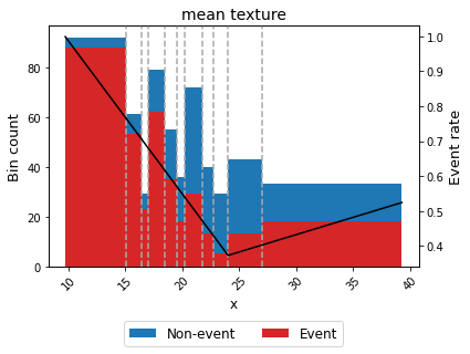
../_images/tutorials_tutorial_piecewise_binary_49_0.png

For example, we can force the variable mean texture to be convex with respect to the probability of having breast cancer.

[26]:

optb = OptimalPWBinning(name=variable, estimator=GradientBoostingClassifier(),
                        monotonic_trend="convex")
optb.fit(x, y, lb=0.001, ub=0.999)

[26]:

OptimalPWBinning(estimator=GradientBoostingClassifier(),
                 monotonic_trend='convex', name='mean texture')

In a Jupyter environment, please rerun this cell to show the HTML representation or trust the notebook.
On GitHub, the HTML representation is unable to render, please try loading this page with nbviewer.org.

[27]:

binning_table = optb.binning_table
binning_table.build()
binning_table.plot(metric="event_rate")

../_images/tutorials_tutorial_piecewise_binary_52_0.png

User-defined split points

In some situations, we have defined split points or bins required to satisfy a priori belief, knowledge or business constraint. The OptimalPWBinning permits to pass user-defined split points. The supplied information is used as a pre-binning, disallowing any pre-binning method set by the user. Furthermore, version 0.5.0 introduces user_splits_fixed parameter, to allow the user to fix some user-defined splits, so these must appear in the solution.

Example numerical variable:

[28]:

user_splits =       [  14,    15,    16,    17,    20,    21,    22,    27]
user_splits_fixed = [False, True,  True, False, False, False, False, False]

[29]:

optb = OptimalPWBinning(name=variable, user_splits=user_splits,
                        user_splits_fixed=user_splits_fixed)

optb.fit(x, y)

[29]:

OptimalPWBinning(estimator=LogisticRegression(), name='mean texture',
                 user_splits=[14, 15, 16, 17, 20, 21, 22, 27],
                 user_splits_fixed=[False, True, True, False, False, False,
                                    False, False])

In a Jupyter environment, please rerun this cell to show the HTML representation or trust the notebook.
On GitHub, the HTML representation is unable to render, please try loading this page with nbviewer.org.

[30]:

binning_table = optb.binning_table
binning_table.build()

[30]:

	Bin	Count	Count (%)	Non-event	Event	c0	c1
0	(-inf, 14.00)	54	0.094903	2	52	1.154009	-0.020568
1	[14.00, 15.00)	37	0.065026	2	35	1.353911	-0.034847
2	[15.00, 16.00)	43	0.075571	7	36	1.247073	-0.027724
3	[16.00, 20.00)	210	0.369069	59	151	1.569012	-0.047846
4	[20.00, 21.00)	45	0.079086	26	19	1.937899	-0.06629
5	[21.00, 22.00)	49	0.086116	30	19	1.54374	-0.047521
6	[22.00, 27.00)	99	0.173989	71	28	1.893766	-0.063431
7	[27.00, inf)	32	0.056239	15	17	0.181134	0.0
8	Special	0	0.000000	0	0	0.0	0.0
9	Missing	0	0.000000	0	0	0.0	0.0
Totals		569	1.000000	212	357	-	-

[31]:

optb.information()

optbinning (Version 1.0.0)
Copyright (c) 2019-2026 Guillermo Navas-Palencia, Apache License 2.0

  Name    : mean texture
  Status  : OPTIMAL

  Pre-binning statistics
    Number of bins                         8

  Solver statistics
    Type                                auto
    Number of variables                   16
    Number of constraints                 23

  Timing
    Total time                          0.16 sec
    Pre-processing                      0.00 sec   (  0.63%)
    Estimator                           0.02 sec   ( 11.38%)
    Pre-binning                         0.08 sec   ( 54.53%)
    Solver                              0.03 sec   ( 19.61%)
    Post-processing                     0.02 sec   ( 12.95%)

Performance: choosing a solver

OptimalPWBinning uses the RoPWR library to solving the piecewise regression problem. See https://github.com/guillermo-navas-palencia/ropwr for details.

Robustness: choosing an objective function and regularization

OptimalPWBinning uses the RoPWR library to solving the piecewise regression problem. See https://github.com/guillermo-navas-palencia/ropwr for details.

Missing data and special codes

For this example, let’s load data from the FICO Explainable Machine Learning Challenge: https://community.fico.com/s/explainable-machine-learning-challenge

[32]:

df = pd.read_csv("data/FICO_challenge/heloc_dataset_v1.csv", sep=",")

The data dictionary of this challenge includes three special values/codes:

-9 No Bureau Record or No Investigation
-8 No Usable/Valid Trades or Inquiries
-7 Condition not Met (e.g. No Inquiries, No Delinquencies)

Version 0.16.0 added support to treat special codes separately.

[33]:

special_codes = {'special_9': -9, 'special_8': -8, 'special_7': -7}

[34]:

variable = "AverageMInFile"
x = df[variable].values.copy()
y = df.RiskPerformance.values

[35]:

df.RiskPerformance.unique()

[35]:

<StringArray>
['Bad', 'Good']
Length: 2, dtype: str

Target is a categorical dichotomic variable, which can be easily transform into numerical.

[36]:

mask = y == "Bad"
y = mask.astype(int)

[37]:

x[10:20] = -8
x[100:105] = -7

For the sake of completeness, we include a few missing values

[38]:

idx = np.random.randint(0, len(x), 500)
x = x.astype(float)
x[idx] = np.nan

[39]:

optb = OptimalPWBinning(name=variable, special_codes=special_codes, solver="osqp")

optb.fit(x, y, lb=0, ub=1)

[39]:

OptimalPWBinning(estimator=LogisticRegression(), name='AverageMInFile',
                 solver='osqp',
                 special_codes={'special_7': -7, 'special_8': -8,
                                'special_9': -9})

In a Jupyter environment, please rerun this cell to show the HTML representation or trust the notebook.
On GitHub, the HTML representation is unable to render, please try loading this page with nbviewer.org.

[40]:

optb.information(print_level=1)

optbinning (Version 1.0.0)
Copyright (c) 2019-2026 Guillermo Navas-Palencia, Apache License 2.0

  Name    : AverageMInFile
  Status  : OPTIMAL

  Pre-binning statistics
    Number of bins                        12

  Solver statistics
    Type                                osqp
    Number of variables                   24
    Number of constraints                 39

  Timing
    Total time                          0.34 sec
    Pre-processing                      0.00 sec   (  1.19%)
    Estimator                           0.05 sec   ( 13.51%)
    Pre-binning                         0.21 sec   ( 61.24%)
    Solver                              0.03 sec   (  9.04%)
    Post-processing                     0.05 sec   ( 14.15%)

[41]:

binning_table = optb.binning_table
binning_table.build()

[41]:

	Bin	Count	Count (%)	Non-event	Event	c0	c1
0	(-inf, 30.50)	548	0.052395	95	453	0.791991	-0.003076
1	[30.50, 41.50)	549	0.052491	148	401	0.804109	-0.003473
2	[41.50, 48.50)	510	0.048762	146	364	0.808176	-0.003571
3	[48.50, 54.50)	525	0.050196	180	345	0.813653	-0.003684
4	[54.50, 59.50)	483	0.046180	198	285	0.817621	-0.003757
5	[59.50, 64.50)	602	0.057558	261	341	0.819753	-0.003793
6	[64.50, 69.50)	648	0.061956	299	349	0.826993	-0.003905
7	[69.50, 74.50)	679	0.064920	324	355	0.812736	-0.0037
8	[74.50, 80.50)	770	0.073621	400	370	0.870012	-0.004469
9	[80.50, 97.50)	1816	0.173630	1029	787	0.777589	-0.003321
10	[97.50, 116.50)	1173	0.112152	719	454	1.0448	-0.006061
11	[116.50, inf)	1092	0.104408	708	384	0.486695	-0.001271
12	special_9	560	0.053542	253	307	0.548214	0.0
13	special_8	10	0.000956	2	8	0.8	0.0
14	special_7	5	0.000478	2	3	0.6	0.0
15	Missing	489	0.046754	236	253	0.517382	0.0
Totals		10459	1.000000	5000	5459	-	-

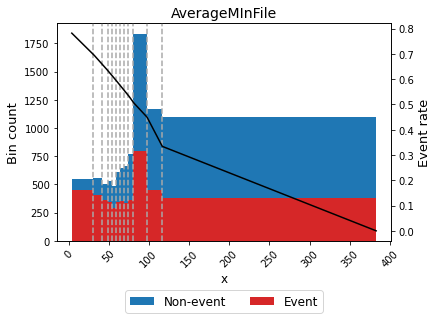
Note the dashed bins 10 and 11, corresponding to the special codes bin and the missing bin, respectively.

[42]:

binning_table.plot(metric="event_rate")

../_images/tutorials_tutorial_piecewise_binary_81_0.png

Verbosity option

For debugging purposes, we can print information on each step of the computation by triggering the verbose option.

[43]:

optb = OptimalPWBinning(name=variable, solver="osqp", verbose=True)
optb.fit(x, y, lb=0, ub=1)

2026-09-12 18:33:41,517 | INFO : Optimal piecewise binning started.
2026-09-12 18:33:41,520 | INFO : Options: check parameters.
2026-09-12 18:33:41,522 | INFO : Pre-processing started.
2026-09-12 18:33:41,523 | INFO : Pre-processing: number of samples: 10459
2026-09-12 18:33:41,526 | INFO : Pre-processing: number of clean samples: 9970
2026-09-12 18:33:41,527 | INFO : Pre-processing: number of missing samples: 489
2026-09-12 18:33:41,529 | INFO : Pre-processing: number of special samples: 0
2026-09-12 18:33:41,534 | INFO : Pre-processing terminated. Time: 0.0007s
2026-09-12 18:33:41,536 | INFO : Pre-binning: set logistic regression as an estimator.
2026-09-12 18:33:41,538 | INFO : Pre-binning: estimator fitting started.
2026-09-12 18:33:41,588 | INFO : Pre-binning: estimator terminated. Time 0.0517s.
2026-09-12 18:33:41,590 | INFO : Pre-binning: optimal binning started.
2026-09-12 18:33:41,726 | INFO : Pre-binning: number of splits: 8.
2026-09-12 18:33:41,728 | INFO : Pre-binning: no need for subsamples.
2026-09-12 18:33:41,729 | INFO : Pre-binning: optimal binning terminated. Time 0.1366s.
2026-09-12 18:33:41,731 | INFO : Optimizer started.
2026-09-12 18:33:41,735 | INFO : Optimizer: descending monotonic trend.

(CVXPY) Sep 12 06:33:41 PM: Your problem has 18 variables, 30 constraints, and 0 parameters.
(CVXPY) Sep 12 06:33:41 PM: It is compliant with the following grammars: DCP, DQCP
(CVXPY) Sep 12 06:33:41 PM: DCP verification time: 0.0003 seconds.
(CVXPY) Sep 12 06:33:41 PM: Expression tree has 4 nodes.
(CVXPY) Sep 12 06:33:41 PM: (If you need to solve this problem multiple times, but with different data, consider using parameters.)
(CVXPY) Sep 12 06:33:41 PM: CVXPY will first compile your problem; then, it will invoke a numerical solver to obtain a solution.
(CVXPY) Sep 12 06:33:41 PM: Your problem is compiled with the CPP canonicalization backend.
(CVXPY) Sep 12 06:33:41 PM: Compiling problem (target solver=OSQP).
(CVXPY) Sep 12 06:33:41 PM: Reduction chain: Dcp2Cone -> CvxAttr2Constr -> EliminateZeroSized -> ConeMatrixStuffing -> OSQP
(CVXPY) Sep 12 06:33:41 PM: Applying reduction Dcp2Cone
(CVXPY) Sep 12 06:33:41 PM: Applying reduction CvxAttr2Constr
(CVXPY) Sep 12 06:33:41 PM: Applying reduction EliminateZeroSized
(CVXPY) Sep 12 06:33:41 PM: Applying reduction ConeMatrixStuffing
(CVXPY) Sep 12 06:33:41 PM: Applying reduction OSQP

===============================================================================
                                     CVXPY
                                     v1.9.2
===============================================================================
-------------------------------------------------------------------------------
                                  Compilation
-------------------------------------------------------------------------------

(CVXPY) Sep 12 06:33:41 PM: Finished problem compilation (took 5.283e-02 seconds).
(CVXPY) Sep 12 06:33:41 PM: Invoking solver OSQP  to obtain a solution.
(CVXPY) Sep 12 06:33:41 PM: Problem status: optimal
(CVXPY) Sep 12 06:33:41 PM: Optimal value: -2.827e+03
(CVXPY) Sep 12 06:33:41 PM: Compilation took 5.283e-02 seconds
(CVXPY) Sep 12 06:33:41 PM: Solver (including time spent in interface) took 7.961e-03 seconds

-------------------------------------------------------------------------------
                                Numerical solver
-------------------------------------------------------------------------------
-----------------------------------------------------------------
           OSQP v1.0.0  -  Operator Splitting QP Solver
              (c) The OSQP Developer Team
-----------------------------------------------------------------
problem:  variables n = 18, constraints m = 30
          nnz(P) + nnz(A) = 76
settings: algebra = Built-in,
          OSQPInt = 4 bytes, OSQPFloat = 8 bytes,
          linear system solver = QDLDL v0.1.8,
          eps_abs = 1.0e-05, eps_rel = 1.0e-05,
          eps_prim_inf = 1.0e-04, eps_dual_inf = 1.0e-04,
          rho = 1.00e-01 (adaptive: 50 iterations),
          sigma = 1.00e-06, alpha = 1.60, max_iter = 10000
          check_termination: on (interval 25, duality gap: on),
          time_limit: 1.00e+10 sec,
          scaling: on (10 iterations), scaled_termination: off
          warm starting: on, polishing: on,
iter   objective    prim res   dual res   gap        rel kkt    rho         time
   1  -1.9836e+03   6.62e-03   9.22e+04   4.27e+03   9.22e+04   1.00e-01    1.36e-04s
  75  -2.8271e+03   3.48e-06   1.22e+00  -1.08e-03   1.22e+00   1.00e-01    3.09e-04s
plsh  -2.8271e+03   1.13e-16   4.45e-11  -8.53e-13   4.45e-11   --------    6.00e-04s

status:               solved
solution polishing:   successful
number of iterations: 75
optimal objective:    -2827.0522
dual objective:       -2827.0522
duality gap:          -8.5324e-13
primal-dual integral: 4.2741e+03
run time:             6.00e-04s
optimal rho estimate: 2.74e-02

-------------------------------------------------------------------------------
                                    Summary
-------------------------------------------------------------------------------
2026-09-12 18:33:41,857 | INFO : Optimizer terminated. Time: 0.1201s
2026-09-12 18:33:41,868 | INFO : Post-processing started.
2026-09-12 18:33:41,871 | INFO : Post-processing: compute binning information.
2026-09-12 18:33:41,878 | INFO : Post-processing: compute performance metrics.
2026-09-12 18:33:41,916 | INFO : Post-processing terminated. Time: 0.0437s
2026-09-12 18:33:41,918 | INFO : Optimal piecewise binning terminated. Status: OPTIMAL. Time: 0.4008s

[43]:

OptimalPWBinning(estimator=LogisticRegression(), name='AverageMInFile',
                 solver='osqp', verbose=True)

In a Jupyter environment, please rerun this cell to show the HTML representation or trust the notebook.
On GitHub, the HTML representation is unable to render, please try loading this page with nbviewer.org.

	penalty penalty: {'l1', 'l2', 'elasticnet', None}, default='l2' Specify the norm of the penalty: - `None`: no penalty is added; - `'l2'`: add an L2 penalty term and it is the default choice; - `'l1'`: add an L1 penalty term; - `'elasticnet'`: both L1 and L2 penalty terms are added. .. warning:: Some penalties may not work with some solvers. See the parameter `solver` below, to know the compatibility between the penalty and solver. .. versionadded:: 0.19 l1 penalty with SAGA solver (allowing 'multinomial' + L1) .. deprecated:: 1.8 `penalty` was deprecated in version 1.8 and will be removed in 1.10. Use `l1_ratio` and `C` instead. `l1_ratio=0` for `penalty='l2'`, `l1_ratio=1` for `penalty='l1'`, `l1_ratio` set to any float between 0 and 1 for `penalty='elasticnet'`, and `C=np.inf` for `penalty=None`.	'deprecated'
	C C: float, default=1.0 Inverse of regularization strength; must be a positive float. Like in support vector machines, smaller values specify stronger regularization. `C=np.inf` results in unpenalized logistic regression. For a visual example on the effect of tuning the `C` parameter with an L1 penalty, see: :ref:`sphx_glr_auto_examples_linear_model_plot_logistic_path.py`.	1.0
	l1_ratio l1_ratio: float, default=0.0 The Elastic-Net mixing parameter, with `0 <= l1_ratio <= 1`. Setting `l1_ratio=1` gives a pure L1-penalty, setting `l1_ratio=0` a pure L2-penalty. Any value between 0 and 1 gives an Elastic-Net penalty of the form `l1_ratio * L1 + (1 - l1_ratio) * L2`. .. warning:: Certain values of `l1_ratio`, i.e. some penalties, may not work with some solvers. See the parameter `solver` below, to know the compatibility between the penalty and solver. .. versionchanged:: 1.8 Default value changed from None to 0.0. .. deprecated:: 1.8 `None` is deprecated and will be removed in version 1.10. Always use `l1_ratio` to specify the penalty type.	0.0
	dual dual: bool, default=False Dual (constrained) or primal (regularized, see also :ref:`this equation <regularized-logistic-loss>`) formulation. Dual formulation is only implemented for l2 penalty with liblinear solver. Prefer `dual=False` when n_samples > n_features.	False
	tol tol: float, default=1e-4 Tolerance for stopping criteria.	0.0001
	fit_intercept fit_intercept: bool, default=True Specifies if a constant (a.k.a. bias or intercept) should be added to the decision function.	True
	intercept_scaling intercept_scaling: float, default=1 Useful only when the solver `liblinear` is used and `self.fit_intercept` is set to `True`. In this case, `x` becomes `[x, self.intercept_scaling]`, i.e. a "synthetic" feature with constant value equal to `intercept_scaling` is appended to the instance vector. The intercept becomes ``intercept_scaling * synthetic_feature_weight``. .. note:: The synthetic feature weight is subject to L1 or L2 regularization as all other features. To lessen the effect of regularization on synthetic feature weight (and therefore on the intercept) `intercept_scaling` has to be increased.	1
	class_weight class_weight: dict or 'balanced', default=None Weights associated with classes in the form ``{class_label: weight}``. If not given, all classes are supposed to have weight one. The "balanced" mode uses the values of y to automatically adjust weights inversely proportional to class frequencies in the input data as ``n_samples / (n_classes * np.bincount(y))``. Note that these weights will be multiplied with sample_weight (passed through the fit method) if sample_weight is specified. .. versionadded:: 0.17 class_weight='balanced'	None
	random_state random_state: int, RandomState instance, default=None Only used for `solver` == 'sag', 'saga' or 'liblinear' to shuffle the data. It has no effect on the other solvers. See :term:`Glossary <random_state>` for details.	None
	solver solver: {'lbfgs', 'liblinear', 'newton-cg', 'newton-cholesky', 'sag', 'saga'}, default='lbfgs' Algorithm to use in the optimization problem. Default is 'lbfgs'. To choose a solver, you might want to consider the following aspects: - 'lbfgs' is a good default solver because it works reasonably well for a wide class of problems. - For :term:`multiclass` problems (`n_classes >= 3`), all solvers except 'liblinear' minimize the full multinomial loss, 'liblinear' will raise an error. - 'newton-cholesky' is a good choice for `n_samples` >> `n_features * n_classes`, especially with one-hot encoded categorical features with rare categories. Be aware that the memory usage of this solver has a quadratic dependency on `n_features * n_classes` because it explicitly computes the full Hessian matrix. - For small datasets, 'liblinear' is a good choice, whereas 'sag' and 'saga' are faster for large ones; - 'liblinear' can only handle binary classification by default. To apply a one-versus-rest scheme for the multiclass setting one can wrap it with the :class:`~sklearn.multiclass.OneVsRestClassifier`. .. warning:: The choice of the algorithm depends on the penalty chosen (`l1_ratio=0` for L2-penalty, `l1_ratio=1` for L1-penalty and `0 < l1_ratio < 1` for Elastic-Net) and on (multinomial) multiclass support: ================= ======================== ====================== solver l1_ratio multinomial multiclass ================= ======================== ====================== 'lbfgs' l1_ratio=0 yes 'liblinear' l1_ratio=1 or l1_ratio=0 no 'newton-cg' l1_ratio=0 yes 'newton-cholesky' l1_ratio=0 yes 'sag' l1_ratio=0 yes 'saga' 0<=l1_ratio<=1 yes ================= ======================== ====================== .. note:: 'sag' and 'saga' fast convergence is only guaranteed on features with approximately the same scale. You can preprocess the data with a scaler from :mod:`sklearn.preprocessing`. .. seealso:: Refer to the :ref:`User Guide <Logistic_regression>` for more information regarding :class:`LogisticRegression` and more specifically the :ref:`Table <logistic_regression_solvers>` summarizing solver/penalty supports. .. versionadded:: 0.17 Stochastic Average Gradient (SAG) descent solver. Multinomial support in version 0.18. .. versionadded:: 0.19 SAGA solver. .. versionchanged:: 0.22 The default solver changed from 'liblinear' to 'lbfgs' in 0.22. .. versionadded:: 1.2 newton-cholesky solver. Multinomial support in version 1.6.	'lbfgs'
	max_iter max_iter: int, default=100 Maximum number of iterations taken for the solvers to converge.	100
	verbose verbose: int, default=0 For the liblinear and lbfgs solvers set verbose to any positive number for verbosity.	0
	warm_start warm_start: bool, default=False When set to True, reuse the solution of the previous call to fit as initialization, otherwise, just erase the previous solution. Useless for liblinear solver. See :term:`the Glossary <warm_start>`. .. versionadded:: 0.17 warm_start to support lbfgs, newton-cg, sag, saga solvers.	False
	n_jobs n_jobs: int, default=None Does not have any effect. .. deprecated:: 1.8 `n_jobs` is deprecated in version 1.8 and will be removed in 1.10.	None

	penalty penalty: {'l1', 'l2', 'elasticnet', None}, default='l2' Specify the norm of the penalty: - `None`: no penalty is added; - `'l2'`: add an L2 penalty term and it is the default choice; - `'l1'`: add an L1 penalty term; - `'elasticnet'`: both L1 and L2 penalty terms are added. .. warning:: Some penalties may not work with some solvers. See the parameter `solver` below, to know the compatibility between the penalty and solver. .. versionadded:: 0.19 l1 penalty with SAGA solver (allowing 'multinomial' + L1) .. deprecated:: 1.8 `penalty` was deprecated in version 1.8 and will be removed in 1.10. Use `l1_ratio` and `C` instead. `l1_ratio=0` for `penalty='l2'`, `l1_ratio=1` for `penalty='l1'`, `l1_ratio` set to any float between 0 and 1 for `penalty='elasticnet'`, and `C=np.inf` for `penalty=None`.	'deprecated'
	C C: float, default=1.0 Inverse of regularization strength; must be a positive float. Like in support vector machines, smaller values specify stronger regularization. `C=np.inf` results in unpenalized logistic regression. For a visual example on the effect of tuning the `C` parameter with an L1 penalty, see: :ref:`sphx_glr_auto_examples_linear_model_plot_logistic_path.py`.	1.0
	l1_ratio l1_ratio: float, default=0.0 The Elastic-Net mixing parameter, with `0 <= l1_ratio <= 1`. Setting `l1_ratio=1` gives a pure L1-penalty, setting `l1_ratio=0` a pure L2-penalty. Any value between 0 and 1 gives an Elastic-Net penalty of the form `l1_ratio * L1 + (1 - l1_ratio) * L2`. .. warning:: Certain values of `l1_ratio`, i.e. some penalties, may not work with some solvers. See the parameter `solver` below, to know the compatibility between the penalty and solver. .. versionchanged:: 1.8 Default value changed from None to 0.0. .. deprecated:: 1.8 `None` is deprecated and will be removed in version 1.10. Always use `l1_ratio` to specify the penalty type.	0.0
	dual dual: bool, default=False Dual (constrained) or primal (regularized, see also :ref:`this equation <regularized-logistic-loss>`) formulation. Dual formulation is only implemented for l2 penalty with liblinear solver. Prefer `dual=False` when n_samples > n_features.	False
	tol tol: float, default=1e-4 Tolerance for stopping criteria.	0.0001
	fit_intercept fit_intercept: bool, default=True Specifies if a constant (a.k.a. bias or intercept) should be added to the decision function.	True
	intercept_scaling intercept_scaling: float, default=1 Useful only when the solver `liblinear` is used and `self.fit_intercept` is set to `True`. In this case, `x` becomes `[x, self.intercept_scaling]`, i.e. a "synthetic" feature with constant value equal to `intercept_scaling` is appended to the instance vector. The intercept becomes ``intercept_scaling * synthetic_feature_weight``. .. note:: The synthetic feature weight is subject to L1 or L2 regularization as all other features. To lessen the effect of regularization on synthetic feature weight (and therefore on the intercept) `intercept_scaling` has to be increased.	1
	class_weight class_weight: dict or 'balanced', default=None Weights associated with classes in the form ``{class_label: weight}``. If not given, all classes are supposed to have weight one. The "balanced" mode uses the values of y to automatically adjust weights inversely proportional to class frequencies in the input data as ``n_samples / (n_classes * np.bincount(y))``. Note that these weights will be multiplied with sample_weight (passed through the fit method) if sample_weight is specified. .. versionadded:: 0.17 class_weight='balanced'	None
	random_state random_state: int, RandomState instance, default=None Only used for `solver` == 'sag', 'saga' or 'liblinear' to shuffle the data. It has no effect on the other solvers. See :term:`Glossary <random_state>` for details.	None
	solver solver: {'lbfgs', 'liblinear', 'newton-cg', 'newton-cholesky', 'sag', 'saga'}, default='lbfgs' Algorithm to use in the optimization problem. Default is 'lbfgs'. To choose a solver, you might want to consider the following aspects: - 'lbfgs' is a good default solver because it works reasonably well for a wide class of problems. - For :term:`multiclass` problems (`n_classes >= 3`), all solvers except 'liblinear' minimize the full multinomial loss, 'liblinear' will raise an error. - 'newton-cholesky' is a good choice for `n_samples` >> `n_features * n_classes`, especially with one-hot encoded categorical features with rare categories. Be aware that the memory usage of this solver has a quadratic dependency on `n_features * n_classes` because it explicitly computes the full Hessian matrix. - For small datasets, 'liblinear' is a good choice, whereas 'sag' and 'saga' are faster for large ones; - 'liblinear' can only handle binary classification by default. To apply a one-versus-rest scheme for the multiclass setting one can wrap it with the :class:`~sklearn.multiclass.OneVsRestClassifier`. .. warning:: The choice of the algorithm depends on the penalty chosen (`l1_ratio=0` for L2-penalty, `l1_ratio=1` for L1-penalty and `0 < l1_ratio < 1` for Elastic-Net) and on (multinomial) multiclass support: ================= ======================== ====================== solver l1_ratio multinomial multiclass ================= ======================== ====================== 'lbfgs' l1_ratio=0 yes 'liblinear' l1_ratio=1 or l1_ratio=0 no 'newton-cg' l1_ratio=0 yes 'newton-cholesky' l1_ratio=0 yes 'sag' l1_ratio=0 yes 'saga' 0<=l1_ratio<=1 yes ================= ======================== ====================== .. note:: 'sag' and 'saga' fast convergence is only guaranteed on features with approximately the same scale. You can preprocess the data with a scaler from :mod:`sklearn.preprocessing`. .. seealso:: Refer to the :ref:`User Guide <Logistic_regression>` for more information regarding :class:`LogisticRegression` and more specifically the :ref:`Table <logistic_regression_solvers>` summarizing solver/penalty supports. .. versionadded:: 0.17 Stochastic Average Gradient (SAG) descent solver. Multinomial support in version 0.18. .. versionadded:: 0.19 SAGA solver. .. versionchanged:: 0.22 The default solver changed from 'liblinear' to 'lbfgs' in 0.22. .. versionadded:: 1.2 newton-cholesky solver. Multinomial support in version 1.6.	'lbfgs'
	max_iter max_iter: int, default=100 Maximum number of iterations taken for the solvers to converge.	100
	verbose verbose: int, default=0 For the liblinear and lbfgs solvers set verbose to any positive number for verbosity.	0
	warm_start warm_start: bool, default=False When set to True, reuse the solution of the previous call to fit as initialization, otherwise, just erase the previous solution. Useless for liblinear solver. See :term:`the Glossary <warm_start>`. .. versionadded:: 0.17 warm_start to support lbfgs, newton-cg, sag, saga solvers.	False
	n_jobs n_jobs: int, default=None Does not have any effect. .. deprecated:: 1.8 `n_jobs` is deprecated in version 1.8 and will be removed in 1.10.	None

	loss loss: {'log_loss', 'exponential'}, default='log_loss' The loss function to be optimized. 'log_loss' refers to binomial and multinomial deviance, the same as used in logistic regression. It is a good choice for classification with probabilistic outputs. For loss 'exponential', gradient boosting recovers the AdaBoost algorithm.	'log_loss'
	learning_rate learning_rate: float, default=0.1 Learning rate shrinks the contribution of each tree by `learning_rate`. There is a trade-off between learning_rate and n_estimators. Values must be in the range `[0.0, inf)`. For an example of the effects of this parameter and its interaction with ``subsample``, see :ref:`sphx_glr_auto_examples_ensemble_plot_gradient_boosting_regularization.py`.	0.1
	n_estimators n_estimators: int, default=100 The number of boosting stages to perform. Gradient boosting is fairly robust to over-fitting so a large number usually results in better performance. Values must be in the range `[1, inf)`.	100
	subsample subsample: float, default=1.0 The fraction of samples to be used for fitting the individual base learners. If smaller than 1.0 this results in Stochastic Gradient Boosting. `subsample` interacts with the parameter `n_estimators`. Choosing `subsample < 1.0` leads to a reduction of variance and an increase in bias. Values must be in the range `(0.0, 1.0]`.	1.0
	criterion criterion: {'friedman_mse', 'squared_error'}, default='friedman_mse' This parameter has no effect. .. versionadded:: 0.18 .. deprecated:: 1.9 `criterion` is deprecated and will be removed in 1.11.	'deprecated'
	min_samples_split min_samples_split: int or float, default=2 The minimum number of samples required to split an internal node: - If int, values must be in the range `[2, inf)`. - If float, values must be in the range `(0.0, 1.0]` and `min_samples_split` will be `ceil(min_samples_split * n_samples)`. .. versionchanged:: 0.18 Added float values for fractions.	2
	min_samples_leaf min_samples_leaf: int or float, default=1 The minimum number of samples required to be at a leaf node. A split point at any depth will only be considered if it leaves at least ``min_samples_leaf`` training samples in each of the left and right branches. This may have the effect of smoothing the model, especially in regression. - If int, values must be in the range `[1, inf)`. - If float, values must be in the range `(0.0, 1.0)` and `min_samples_leaf` will be `ceil(min_samples_leaf * n_samples)`. .. versionchanged:: 0.18 Added float values for fractions.	1
	min_weight_fraction_leaf min_weight_fraction_leaf: float, default=0.0 The minimum weighted fraction of the sum total of weights (of all the input samples) required to be at a leaf node. Samples have equal weight when sample_weight is not provided. Values must be in the range `[0.0, 0.5]`.	0.0
	max_depth max_depth: int or None, default=3 Maximum depth of the individual regression estimators. The maximum depth limits the number of nodes in the tree. Tune this parameter for best performance; the best value depends on the interaction of the input variables. If None, then nodes are expanded until all leaves are pure or until all leaves contain less than min_samples_split samples. If int, values must be in the range `[1, inf)`.	3
	min_impurity_decrease min_impurity_decrease: float, default=0.0 A node will be split if this split induces a decrease of the impurity greater than or equal to this value. Values must be in the range `[0.0, inf)`. The weighted impurity decrease equation is the following:: N_t / N * (impurity - N_t_R / N_t * right_impurity - N_t_L / N_t * left_impurity) where ``N`` is the total number of samples, ``N_t`` is the number of samples at the current node, ``N_t_L`` is the number of samples in the left child, and ``N_t_R`` is the number of samples in the right child. ``N``, ``N_t``, ``N_t_R`` and ``N_t_L`` all refer to the weighted sum, if ``sample_weight`` is passed. .. versionadded:: 0.19	0.0
	init init: estimator or 'zero', default=None An estimator object that is used to compute the initial predictions. ``init`` has to provide :term:`fit` and :term:`predict_proba`. If 'zero', the initial raw predictions are set to zero. By default, a ``DummyEstimator`` predicting the classes priors is used.	None
	random_state random_state: int, RandomState instance or None, default=None Controls the random seed given to each Tree estimator at each boosting iteration. In addition, it controls the random permutation of the features at each split (see Notes for more details). It also controls the random splitting of the training data to obtain a validation set if `n_iter_no_change` is not None. Pass an int for reproducible output across multiple function calls. See :term:`Glossary <random_state>`.	None
	max_features max_features: {'sqrt', 'log2'}, int or float, default=None The number of features to consider when looking for the best split: - If int, values must be in the range `[1, inf)`. - If float, values must be in the range `(0.0, 1.0]` and the features considered at each split will be `max(1, int(max_features * n_features_in_))`. - If 'sqrt', then `max_features=sqrt(n_features)`. - If 'log2', then `max_features=log2(n_features)`. - If None, then `max_features=n_features`. Choosing `max_features < n_features` leads to a reduction of variance and an increase in bias. Note: the search for a split does not stop until at least one valid partition of the node samples is found, even if it requires to effectively inspect more than ``max_features`` features.	None
	verbose verbose: int, default=0 Enable verbose output. If 1 then it prints progress and performance once in a while (the more trees the lower the frequency). If greater than 1 then it prints progress and performance for every tree. Values must be in the range `[0, inf)`.	0
	max_leaf_nodes max_leaf_nodes: int, default=None Grow trees with ``max_leaf_nodes`` in best-first fashion. Best nodes are defined as relative reduction in impurity. Values must be in the range `[2, inf)`. If `None`, then unlimited number of leaf nodes.	None
	warm_start warm_start: bool, default=False When set to ``True``, reuse the solution of the previous call to fit and add more estimators to the ensemble, otherwise, just erase the previous solution. See :term:`the Glossary <warm_start>`.	False
	validation_fraction validation_fraction: float, default=0.1 The proportion of training data to set aside as validation set for early stopping. Values must be in the range `(0.0, 1.0)`. Only used if ``n_iter_no_change`` is set to an integer. .. versionadded:: 0.20	0.1
	n_iter_no_change n_iter_no_change: int, default=None ``n_iter_no_change`` is used to decide if early stopping will be used to terminate training when validation score is not improving. By default it is set to None to disable early stopping. If set to a number, it will set aside ``validation_fraction`` size of the training data as validation and terminate training when validation score is not improving in all of the previous ``n_iter_no_change`` numbers of iterations. The split is stratified. Values must be in the range `[1, inf)`. See :ref:`sphx_glr_auto_examples_ensemble_plot_gradient_boosting_early_stopping.py`. .. versionadded:: 0.20	None
	tol tol: float, default=1e-4 Tolerance for the early stopping. When the loss is not improving by at least tol for ``n_iter_no_change`` iterations (if set to a number), the training stops. Values must be in the range `[0.0, inf)`. .. versionadded:: 0.20	0.0001
	ccp_alpha ccp_alpha: non-negative float, default=0.0 Complexity parameter used for Minimal Cost-Complexity Pruning. The subtree with the largest cost complexity that is smaller than ``ccp_alpha`` will be chosen. By default, no pruning is performed. Values must be in the range `[0.0, inf)`. See :ref:`minimal_cost_complexity_pruning` for details. See :ref:`sphx_glr_auto_examples_tree_plot_cost_complexity_pruning.py` for an example of such pruning. .. versionadded:: 0.22	0.0

	loss loss: {'log_loss', 'exponential'}, default='log_loss' The loss function to be optimized. 'log_loss' refers to binomial and multinomial deviance, the same as used in logistic regression. It is a good choice for classification with probabilistic outputs. For loss 'exponential', gradient boosting recovers the AdaBoost algorithm.	'log_loss'
	learning_rate learning_rate: float, default=0.1 Learning rate shrinks the contribution of each tree by `learning_rate`. There is a trade-off between learning_rate and n_estimators. Values must be in the range `[0.0, inf)`. For an example of the effects of this parameter and its interaction with ``subsample``, see :ref:`sphx_glr_auto_examples_ensemble_plot_gradient_boosting_regularization.py`.	0.1
	n_estimators n_estimators: int, default=100 The number of boosting stages to perform. Gradient boosting is fairly robust to over-fitting so a large number usually results in better performance. Values must be in the range `[1, inf)`.	100
	subsample subsample: float, default=1.0 The fraction of samples to be used for fitting the individual base learners. If smaller than 1.0 this results in Stochastic Gradient Boosting. `subsample` interacts with the parameter `n_estimators`. Choosing `subsample < 1.0` leads to a reduction of variance and an increase in bias. Values must be in the range `(0.0, 1.0]`.	1.0
	criterion criterion: {'friedman_mse', 'squared_error'}, default='friedman_mse' This parameter has no effect. .. versionadded:: 0.18 .. deprecated:: 1.9 `criterion` is deprecated and will be removed in 1.11.	'deprecated'
	min_samples_split min_samples_split: int or float, default=2 The minimum number of samples required to split an internal node: - If int, values must be in the range `[2, inf)`. - If float, values must be in the range `(0.0, 1.0]` and `min_samples_split` will be `ceil(min_samples_split * n_samples)`. .. versionchanged:: 0.18 Added float values for fractions.	2
	min_samples_leaf min_samples_leaf: int or float, default=1 The minimum number of samples required to be at a leaf node. A split point at any depth will only be considered if it leaves at least ``min_samples_leaf`` training samples in each of the left and right branches. This may have the effect of smoothing the model, especially in regression. - If int, values must be in the range `[1, inf)`. - If float, values must be in the range `(0.0, 1.0)` and `min_samples_leaf` will be `ceil(min_samples_leaf * n_samples)`. .. versionchanged:: 0.18 Added float values for fractions.	1
	min_weight_fraction_leaf min_weight_fraction_leaf: float, default=0.0 The minimum weighted fraction of the sum total of weights (of all the input samples) required to be at a leaf node. Samples have equal weight when sample_weight is not provided. Values must be in the range `[0.0, 0.5]`.	0.0
	max_depth max_depth: int or None, default=3 Maximum depth of the individual regression estimators. The maximum depth limits the number of nodes in the tree. Tune this parameter for best performance; the best value depends on the interaction of the input variables. If None, then nodes are expanded until all leaves are pure or until all leaves contain less than min_samples_split samples. If int, values must be in the range `[1, inf)`.	3
	min_impurity_decrease min_impurity_decrease: float, default=0.0 A node will be split if this split induces a decrease of the impurity greater than or equal to this value. Values must be in the range `[0.0, inf)`. The weighted impurity decrease equation is the following:: N_t / N * (impurity - N_t_R / N_t * right_impurity - N_t_L / N_t * left_impurity) where ``N`` is the total number of samples, ``N_t`` is the number of samples at the current node, ``N_t_L`` is the number of samples in the left child, and ``N_t_R`` is the number of samples in the right child. ``N``, ``N_t``, ``N_t_R`` and ``N_t_L`` all refer to the weighted sum, if ``sample_weight`` is passed. .. versionadded:: 0.19	0.0
	init init: estimator or 'zero', default=None An estimator object that is used to compute the initial predictions. ``init`` has to provide :term:`fit` and :term:`predict_proba`. If 'zero', the initial raw predictions are set to zero. By default, a ``DummyEstimator`` predicting the classes priors is used.	None
	random_state random_state: int, RandomState instance or None, default=None Controls the random seed given to each Tree estimator at each boosting iteration. In addition, it controls the random permutation of the features at each split (see Notes for more details). It also controls the random splitting of the training data to obtain a validation set if `n_iter_no_change` is not None. Pass an int for reproducible output across multiple function calls. See :term:`Glossary <random_state>`.	None
	max_features max_features: {'sqrt', 'log2'}, int or float, default=None The number of features to consider when looking for the best split: - If int, values must be in the range `[1, inf)`. - If float, values must be in the range `(0.0, 1.0]` and the features considered at each split will be `max(1, int(max_features * n_features_in_))`. - If 'sqrt', then `max_features=sqrt(n_features)`. - If 'log2', then `max_features=log2(n_features)`. - If None, then `max_features=n_features`. Choosing `max_features < n_features` leads to a reduction of variance and an increase in bias. Note: the search for a split does not stop until at least one valid partition of the node samples is found, even if it requires to effectively inspect more than ``max_features`` features.	None
	verbose verbose: int, default=0 Enable verbose output. If 1 then it prints progress and performance once in a while (the more trees the lower the frequency). If greater than 1 then it prints progress and performance for every tree. Values must be in the range `[0, inf)`.	0
	max_leaf_nodes max_leaf_nodes: int, default=None Grow trees with ``max_leaf_nodes`` in best-first fashion. Best nodes are defined as relative reduction in impurity. Values must be in the range `[2, inf)`. If `None`, then unlimited number of leaf nodes.	None
	warm_start warm_start: bool, default=False When set to ``True``, reuse the solution of the previous call to fit and add more estimators to the ensemble, otherwise, just erase the previous solution. See :term:`the Glossary <warm_start>`.	False
	validation_fraction validation_fraction: float, default=0.1 The proportion of training data to set aside as validation set for early stopping. Values must be in the range `(0.0, 1.0)`. Only used if ``n_iter_no_change`` is set to an integer. .. versionadded:: 0.20	0.1
	n_iter_no_change n_iter_no_change: int, default=None ``n_iter_no_change`` is used to decide if early stopping will be used to terminate training when validation score is not improving. By default it is set to None to disable early stopping. If set to a number, it will set aside ``validation_fraction`` size of the training data as validation and terminate training when validation score is not improving in all of the previous ``n_iter_no_change`` numbers of iterations. The split is stratified. Values must be in the range `[1, inf)`. See :ref:`sphx_glr_auto_examples_ensemble_plot_gradient_boosting_early_stopping.py`. .. versionadded:: 0.20	None
	tol tol: float, default=1e-4 Tolerance for the early stopping. When the loss is not improving by at least tol for ``n_iter_no_change`` iterations (if set to a number), the training stops. Values must be in the range `[0.0, inf)`. .. versionadded:: 0.20	0.0001
	ccp_alpha ccp_alpha: non-negative float, default=0.0 Complexity parameter used for Minimal Cost-Complexity Pruning. The subtree with the largest cost complexity that is smaller than ``ccp_alpha`` will be chosen. By default, no pruning is performed. Values must be in the range `[0.0, inf)`. See :ref:`minimal_cost_complexity_pruning` for details. See :ref:`sphx_glr_auto_examples_tree_plot_cost_complexity_pruning.py` for an example of such pruning. .. versionadded:: 0.22	0.0

	penalty penalty: {'l1', 'l2', 'elasticnet', None}, default='l2' Specify the norm of the penalty: - `None`: no penalty is added; - `'l2'`: add an L2 penalty term and it is the default choice; - `'l1'`: add an L1 penalty term; - `'elasticnet'`: both L1 and L2 penalty terms are added. .. warning:: Some penalties may not work with some solvers. See the parameter `solver` below, to know the compatibility between the penalty and solver. .. versionadded:: 0.19 l1 penalty with SAGA solver (allowing 'multinomial' + L1) .. deprecated:: 1.8 `penalty` was deprecated in version 1.8 and will be removed in 1.10. Use `l1_ratio` and `C` instead. `l1_ratio=0` for `penalty='l2'`, `l1_ratio=1` for `penalty='l1'`, `l1_ratio` set to any float between 0 and 1 for `penalty='elasticnet'`, and `C=np.inf` for `penalty=None`.	'deprecated'
	C C: float, default=1.0 Inverse of regularization strength; must be a positive float. Like in support vector machines, smaller values specify stronger regularization. `C=np.inf` results in unpenalized logistic regression. For a visual example on the effect of tuning the `C` parameter with an L1 penalty, see: :ref:`sphx_glr_auto_examples_linear_model_plot_logistic_path.py`.	1.0
	l1_ratio l1_ratio: float, default=0.0 The Elastic-Net mixing parameter, with `0 <= l1_ratio <= 1`. Setting `l1_ratio=1` gives a pure L1-penalty, setting `l1_ratio=0` a pure L2-penalty. Any value between 0 and 1 gives an Elastic-Net penalty of the form `l1_ratio * L1 + (1 - l1_ratio) * L2`. .. warning:: Certain values of `l1_ratio`, i.e. some penalties, may not work with some solvers. See the parameter `solver` below, to know the compatibility between the penalty and solver. .. versionchanged:: 1.8 Default value changed from None to 0.0. .. deprecated:: 1.8 `None` is deprecated and will be removed in version 1.10. Always use `l1_ratio` to specify the penalty type.	0.0
	dual dual: bool, default=False Dual (constrained) or primal (regularized, see also :ref:`this equation <regularized-logistic-loss>`) formulation. Dual formulation is only implemented for l2 penalty with liblinear solver. Prefer `dual=False` when n_samples > n_features.	False
	tol tol: float, default=1e-4 Tolerance for stopping criteria.	0.0001
	fit_intercept fit_intercept: bool, default=True Specifies if a constant (a.k.a. bias or intercept) should be added to the decision function.	True
	intercept_scaling intercept_scaling: float, default=1 Useful only when the solver `liblinear` is used and `self.fit_intercept` is set to `True`. In this case, `x` becomes `[x, self.intercept_scaling]`, i.e. a "synthetic" feature with constant value equal to `intercept_scaling` is appended to the instance vector. The intercept becomes ``intercept_scaling * synthetic_feature_weight``. .. note:: The synthetic feature weight is subject to L1 or L2 regularization as all other features. To lessen the effect of regularization on synthetic feature weight (and therefore on the intercept) `intercept_scaling` has to be increased.	1
	class_weight class_weight: dict or 'balanced', default=None Weights associated with classes in the form ``{class_label: weight}``. If not given, all classes are supposed to have weight one. The "balanced" mode uses the values of y to automatically adjust weights inversely proportional to class frequencies in the input data as ``n_samples / (n_classes * np.bincount(y))``. Note that these weights will be multiplied with sample_weight (passed through the fit method) if sample_weight is specified. .. versionadded:: 0.17 class_weight='balanced'	None
	random_state random_state: int, RandomState instance, default=None Only used for `solver` == 'sag', 'saga' or 'liblinear' to shuffle the data. It has no effect on the other solvers. See :term:`Glossary <random_state>` for details.	None
	solver solver: {'lbfgs', 'liblinear', 'newton-cg', 'newton-cholesky', 'sag', 'saga'}, default='lbfgs' Algorithm to use in the optimization problem. Default is 'lbfgs'. To choose a solver, you might want to consider the following aspects: - 'lbfgs' is a good default solver because it works reasonably well for a wide class of problems. - For :term:`multiclass` problems (`n_classes >= 3`), all solvers except 'liblinear' minimize the full multinomial loss, 'liblinear' will raise an error. - 'newton-cholesky' is a good choice for `n_samples` >> `n_features * n_classes`, especially with one-hot encoded categorical features with rare categories. Be aware that the memory usage of this solver has a quadratic dependency on `n_features * n_classes` because it explicitly computes the full Hessian matrix. - For small datasets, 'liblinear' is a good choice, whereas 'sag' and 'saga' are faster for large ones; - 'liblinear' can only handle binary classification by default. To apply a one-versus-rest scheme for the multiclass setting one can wrap it with the :class:`~sklearn.multiclass.OneVsRestClassifier`. .. warning:: The choice of the algorithm depends on the penalty chosen (`l1_ratio=0` for L2-penalty, `l1_ratio=1` for L1-penalty and `0 < l1_ratio < 1` for Elastic-Net) and on (multinomial) multiclass support: ================= ======================== ====================== solver l1_ratio multinomial multiclass ================= ======================== ====================== 'lbfgs' l1_ratio=0 yes 'liblinear' l1_ratio=1 or l1_ratio=0 no 'newton-cg' l1_ratio=0 yes 'newton-cholesky' l1_ratio=0 yes 'sag' l1_ratio=0 yes 'saga' 0<=l1_ratio<=1 yes ================= ======================== ====================== .. note:: 'sag' and 'saga' fast convergence is only guaranteed on features with approximately the same scale. You can preprocess the data with a scaler from :mod:`sklearn.preprocessing`. .. seealso:: Refer to the :ref:`User Guide <Logistic_regression>` for more information regarding :class:`LogisticRegression` and more specifically the :ref:`Table <logistic_regression_solvers>` summarizing solver/penalty supports. .. versionadded:: 0.17 Stochastic Average Gradient (SAG) descent solver. Multinomial support in version 0.18. .. versionadded:: 0.19 SAGA solver. .. versionchanged:: 0.22 The default solver changed from 'liblinear' to 'lbfgs' in 0.22. .. versionadded:: 1.2 newton-cholesky solver. Multinomial support in version 1.6.	'lbfgs'
	max_iter max_iter: int, default=100 Maximum number of iterations taken for the solvers to converge.	100
	verbose verbose: int, default=0 For the liblinear and lbfgs solvers set verbose to any positive number for verbosity.	0
	warm_start warm_start: bool, default=False When set to True, reuse the solution of the previous call to fit as initialization, otherwise, just erase the previous solution. Useless for liblinear solver. See :term:`the Glossary <warm_start>`. .. versionadded:: 0.17 warm_start to support lbfgs, newton-cg, sag, saga solvers.	False
	n_jobs n_jobs: int, default=None Does not have any effect. .. deprecated:: 1.8 `n_jobs` is deprecated in version 1.8 and will be removed in 1.10.	None