Tutorial: optimal piecewise binning with continuous target
Basic
To get us started, let’s load a well-known dataset from the UCI repository and transform the data into a pandas.DataFrame.
[1]:
import numpy as np
import pandas as pd
[2]:
class Data:
    def __init__(self, data, target, feature_names):
        self.data = data
        self.target = target
        self.feature_names = feature_names


def load_boston():
    data_url = "../../../tests/data/boston_housing.csv"
    raw_df = pd.read_csv(data_url, sep=r"\s+", skiprows=22, header=None)
    raw_data = np.hstack([raw_df.values[::2, :], raw_df.values[1::2, :2]])
    target = raw_df.values[1::2, 2]
    feature_names = ['CRIM', 'ZN', 'INDUS', 'CHAS', 'NOX', 'RM', 'AGE', 'DIS',
                     'RAD', 'TAX', 'PTRATIO', 'B', 'LSTAT']

    return Data(raw_data, target, feature_names)


data = load_boston()
df = pd.DataFrame(data.data, columns=data.feature_names)
We choose a variable to discretize and the continuous target.
[3]:
variable = "LSTAT"
x = df[variable].values
y = data.target
Import and instantiate an ContinuousOptimalPWBinning object class and we pass the variable name. The ContinuousOptimalPWBinning can ONLY handle numerical variables. This differs from the ContinuousOptimalBinning object class.
[4]:
from optbinning import ContinuousOptimalPWBinning
[5]:
optb = ContinuousOptimalPWBinning(name=variable)
We fit the optimal binning object with arrays x and y.
[6]:
optb.fit(x, y)
[6]:
ContinuousOptimalPWBinning(name='LSTAT')In a Jupyter environment, please rerun this cell to show the HTML representation or trust the notebook.
On GitHub, the HTML representation is unable to render, please try loading this page with nbviewer.org.
Parameters
| name | 'LSTAT' | |
| objective | 'l2' | |
| degree | 1 | |
| continuous | True | |
| continuous_deriv | True | |
| prebinning_method | 'cart' | |
| max_n_prebins | 20 | |
| min_prebin_size | 0.05 | |
| min_n_bins | None | |
| max_n_bins | None | |
| min_bin_size | None | |
| max_bin_size | None | |
| monotonic_trend | 'auto' | |
| n_subsamples | None | |
| max_pvalue | None | |
| max_pvalue_policy | 'consecutive' | |
| outlier_detector | None | |
| outlier_params | None | |
| user_splits | None | |
| user_splits_fixed | None | |
| special_codes | None | |
| split_digits | None | |
| solver | 'auto' | |
| h_epsilon | 1.35 | |
| quantile | 0.5 | |
| regularization | None | |
| reg_l1 | 1.0 | |
| reg_l2 | 1.0 | |
| random_state | None | |
| verbose | False |
You can check if an optimal solution has been found via the status attribute:
[7]:
optb.status
[7]:
'OPTIMAL'
You can also retrieve the optimal split points via the splits attribute:
[8]:
optb.splits
[8]:
array([ 4.6500001 ,  5.49499989,  6.86500001,  9.7249999 , 13.0999999 ,
       14.4000001 , 17.23999977, 19.89999962, 23.31500053])
The binning table
The optimal binning algorithms return a binning table; a binning table displays the binned data and several metrics for each bin. Class ContinuousOptimalPWBinning returns an object PWContinuousBinningTable via the binning_table attribute.
[9]:
binning_table = optb.binning_table
[10]:
type(binning_table)
[10]:
optbinning.binning.piecewise.binning_statistics.PWContinuousBinningTable
The binning_table is instantiated, but not built. Therefore, the first step is to call the method build, which returns a pandas.DataFrame.
[11]:
binning_table.build()
[11]:
| Bin | Count | Count (%) | Sum | Std | Min | Max | Zeros count | c0 | c1 | |
|---|---|---|---|---|---|---|---|---|---|---|
| 0 | (-inf, 4.65) | 50.0 | 0.098814 | 1985.9 | 8.198651 | 22.8 | 50.0 | 0 | 56.744159 | -4.821782 |
| 1 | [4.65, 5.49) | 28.0 | 0.055336 | 853.2 | 6.123541 | 21.9 | 50.0 | 0 | 74.661288 | -8.674928 |
| 2 | [5.49, 6.87) | 45.0 | 0.088933 | 1188.6 | 5.136259 | 20.6 | 48.8 | 0 | 26.992559 | 0.0 |
| 3 | [6.87, 9.72) | 89.0 | 0.175889 | 2274.9 | 6.84525 | 11.9 | 50.0 | 0 | 36.39643 | -1.369828 |
| 4 | [9.72, 13.10) | 84.0 | 0.166008 | 1755.4 | 2.949979 | 14.5 | 31.0 | 0 | 31.699082 | -0.88681 |
| 5 | [13.10, 14.40) | 32.0 | 0.063241 | 667.4 | 2.632482 | 15.0 | 29.6 | 0 | 27.030847 | -0.530457 |
| 6 | [14.40, 17.24) | 60.0 | 0.118577 | 1037.5 | 3.588003 | 10.2 | 30.7 | 0 | 35.230335 | -1.099866 |
| 7 | [17.24, 19.90) | 43.0 | 0.084980 | 714.3 | 4.032554 | 8.3 | 27.5 | 0 | 23.261993 | -0.405646 |
| 8 | [19.90, 23.32) | 28.0 | 0.055336 | 368.4 | 3.912839 | 5.0 | 21.7 | 0 | 33.251551 | -0.907634 |
| 9 | [23.32, inf) | 47.0 | 0.092885 | 556.0 | 4.006586 | 5.0 | 23.7 | 0 | 13.222399 | -0.048567 |
| 10 | Special | 0.0 | 0.000000 | 0.0 | None | None | None | 0 | 0.0 | 0.0 |
| 11 | Missing | 0.0 | 0.000000 | 0.0 | None | None | None | 0 | 0.0 | 0.0 |
| Totals | 506.0 | 1.000000 | 11401.6 | 5.0 | 50.0 | 0 | - | - |
Let’s describe the columns of this binning table:
Bin: the intervals delimited by the optimal split points.
Count: the number of records for each bin.
Count (%): the percentage of records for each bin.
Sum: the target sum for each bin.
Std: the target std for each bin.
Min: the target min value for each bin.
Max: the target max value for each bin.
Zeros count: the number of zeros for each bin.
\(c_0\): the first coefficient of the prediction polynomial.
\(c_1\): the second coefficient of the prediction polynomial.
The for bin \(i\) is defined as \(P_i = c_0 + c_1 x_i\), where \(x_i \in \text{Bin}_{i}\). In general, \begin{equation} P_i = \sum_{j=0}^d c_j x_i^j, \end{equation} where \(d\) is the degree of the event rate polynomial.
The last row shows the total number of records, sum and mean.
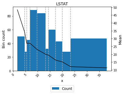
You can use the method plot to visualize the histogram and mean curve.
[12]:
binning_table.plot()
Mean transformation
Now that we have checked the binned data, we can transform our original data into mean values.
[13]:
x_transform_mean = optb.transform(x)
Advanced
Many of the advanced options have been covered in the previous tutorials with a binary target. Check it out! In this section, we focus on the mean monotonicity trend and the mean difference between bins.
Binning table statistical analysis
The analysis method performs a statistical analysis of the binning table, computing the Information Value (IV) and Herfindahl-Hirschman Index (HHI). Additionally, several statistical significance tests between consecutive bins of the contingency table are performed using the Student’s t-test. The piecewise binning also includes several performance metrics for regression problems.
[14]:
binning_table.analysis()
-------------------------------------------------
OptimalBinning: Continuous Binning Table Analysis
-------------------------------------------------

  General metrics

    Mean absolute error              3.67892092
    Mean squared error              26.06425104
    Median absolute error            2.71794570
    Explained variance               0.69125340
    R^2                              0.69125340
    MPE                             -0.05221127
    MAPE                             0.17785599
    SMAPE                            0.08395478
    MdAPE                            0.13052555
    SMdAPE                           0.06542912
    HHI                              0.11620241
    HHI (normalized)                 0.01800268
    Quality score                    0.01702213

  Significance tests

    Bin A  Bin B  t-statistic      p-value
        0      1     5.644492 3.313748e-07
        1      2     2.924528 5.175586e-03
        2      3     0.808313 4.206096e-01
        3      4     5.874488 3.816654e-08
        4      5     0.073112 9.419504e-01
        5      6     5.428848 5.770714e-07
        6      7     0.883289 3.796030e-01
        7      8     3.591859 6.692488e-04
        8      9     1.408305 1.643801e-01
[15]:
binning_table.analysis()
-------------------------------------------------
OptimalBinning: Continuous Binning Table Analysis
-------------------------------------------------

  General metrics

    Mean absolute error              3.67892092
    Mean squared error              26.06425104
    Median absolute error            2.71794570
    Explained variance               0.69125340
    R^2                              0.69125340
    MPE                             -0.05221127
    MAPE                             0.17785599
    SMAPE                            0.08395478
    MdAPE                            0.13052555
    SMdAPE                           0.06542912
    HHI                              0.11620241
    HHI (normalized)                 0.01800268
    Quality score                    0.01702213

  Significance tests

    Bin A  Bin B  t-statistic      p-value
        0      1     5.644492 3.313748e-07
        1      2     2.924528 5.175586e-03
        2      3     0.808313 4.206096e-01
        3      4     5.874488 3.816654e-08
        4      5     0.073112 9.419504e-01
        5      6     5.428848 5.770714e-07
        6      7     0.883289 3.796030e-01
        7      8     3.591859 6.692488e-04
        8      9     1.408305 1.643801e-01
Mean monotonicity
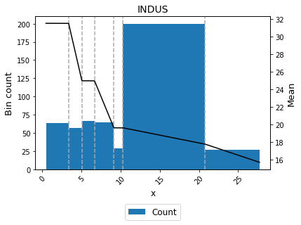
The monotonic_trend option permits forcing a monotonic trend to the mean curve. The default setting “auto” should be the preferred option, however, some business constraints might require to impose different trends. The default setting “auto” chooses the monotonic trend most likely to minimize the L1-norm from the options “ascending”, “descending”, “peak” and “valley” using a machine-learning-based classifier.
[16]:
variable = "INDUS"
x = df[variable].values
y = data.target
[17]:
optb = ContinuousOptimalPWBinning(name=variable, monotonic_trend="auto")
optb.fit(x, y)
[17]:
ContinuousOptimalPWBinning(name='INDUS')In a Jupyter environment, please rerun this cell to show the HTML representation or trust the notebook.
On GitHub, the HTML representation is unable to render, please try loading this page with nbviewer.org.
Parameters
| name | 'INDUS' | |
| objective | 'l2' | |
| degree | 1 | |
| continuous | True | |
| continuous_deriv | True | |
| prebinning_method | 'cart' | |
| max_n_prebins | 20 | |
| min_prebin_size | 0.05 | |
| min_n_bins | None | |
| max_n_bins | None | |
| min_bin_size | None | |
| max_bin_size | None | |
| monotonic_trend | 'auto' | |
| n_subsamples | None | |
| max_pvalue | None | |
| max_pvalue_policy | 'consecutive' | |
| outlier_detector | None | |
| outlier_params | None | |
| user_splits | None | |
| user_splits_fixed | None | |
| special_codes | None | |
| split_digits | None | |
| solver | 'auto' | |
| h_epsilon | 1.35 | |
| quantile | 0.5 | |
| regularization | None | |
| reg_l1 | 1.0 | |
| reg_l2 | 1.0 | |
| random_state | None | |
| verbose | False |
[18]:
binning_table = optb.binning_table
binning_table.build()
[18]:
| Bin | Count | Count (%) | Sum | Std | Min | Max | Zeros count | c0 | c1 | |
|---|---|---|---|---|---|---|---|---|---|---|
| 0 | (-inf, 3.35) | 63.0 | 0.124506 | 1994.0 | 8.569841 | 16.5 | 50.0 | 0 | 31.494243 | 0.0 |
| 1 | [3.35, 5.04) | 57.0 | 0.112648 | 1615.2 | 8.07271 | 17.2 | 50.0 | 0 | 44.441955 | -3.864989 |
| 2 | [5.04, 6.66) | 66.0 | 0.130435 | 1723.7 | 7.879078 | 16.0 | 50.0 | 0 | 24.962412 | 0.0 |
| 3 | [6.66, 9.12) | 64.0 | 0.126482 | 1292.0 | 4.614126 | 12.7 | 35.2 | 0 | 39.414039 | -2.169914 |
| 4 | [9.12, 10.30) | 29.0 | 0.057312 | 584.1 | 2.252281 | 16.1 | 24.5 | 0 | 19.613573 | 0.0 |
| 5 | [10.30, 20.73) | 200.0 | 0.395257 | 3736.2 | 8.959305 | 5.0 | 50.0 | 0 | 21.429532 | -0.176307 |
| 6 | [20.73, inf) | 27.0 | 0.053360 | 456.4 | 3.690878 | 7.0 | 23.0 | 0 | 23.933551 | -0.29707 |
| 7 | Special | 0.0 | 0.000000 | 0.0 | None | None | None | 0 | 0.0 | 0.0 |
| 8 | Missing | 0.0 | 0.000000 | 0.0 | None | None | None | 0 | 0.0 | 0.0 |
| Totals | 506.0 | 1.000000 | 11401.6 | 5.0 | 50.0 | 0 | - | - |
[19]:
binning_table.plot()
[20]:
binning_table.analysis()
-------------------------------------------------
OptimalBinning: Continuous Binning Table Analysis
-------------------------------------------------

  General metrics

    Mean absolute error              5.44142744
    Mean squared error              59.78870565
    Median absolute error            4.13838129
    Explained variance               0.29176712
    R^2                              0.29176712
    MPE                             -0.12274348
    MAPE                             0.28239036
    SMAPE                            0.12302499
    MdAPE                            0.19474014
    SMdAPE                           0.09639011
    HHI                              0.22356231
    HHI (normalized)                 0.09415603
    Quality score                    0.03479317

  Significance tests

    Bin A  Bin B  t-statistic      p-value
        0      1     2.180865 3.118080e-02
        1      2     1.537968 1.267445e-01
        2      3     5.254539 7.781110e-07
        3      4     0.064736 9.485275e-01
        4      5     1.923770 5.601023e-02
        5      6     1.867339 6.563949e-02
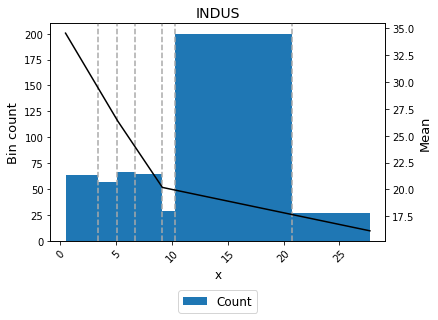
A smoother curve, keeping the valley monotonicity, can be achieved by using monotonic_trend="convex".
[21]:
optb = ContinuousOptimalPWBinning(name=variable, monotonic_trend="convex")
optb.fit(x, y)
[21]:
ContinuousOptimalPWBinning(monotonic_trend='convex', name='INDUS')In a Jupyter environment, please rerun this cell to show the HTML representation or trust the notebook.
On GitHub, the HTML representation is unable to render, please try loading this page with nbviewer.org.
Parameters
| name | 'INDUS' | |
| monotonic_trend | 'convex' | |
| objective | 'l2' | |
| degree | 1 | |
| continuous | True | |
| continuous_deriv | True | |
| prebinning_method | 'cart' | |
| max_n_prebins | 20 | |
| min_prebin_size | 0.05 | |
| min_n_bins | None | |
| max_n_bins | None | |
| min_bin_size | None | |
| max_bin_size | None | |
| n_subsamples | None | |
| max_pvalue | None | |
| max_pvalue_policy | 'consecutive' | |
| outlier_detector | None | |
| outlier_params | None | |
| user_splits | None | |
| user_splits_fixed | None | |
| special_codes | None | |
| split_digits | None | |
| solver | 'auto' | |
| h_epsilon | 1.35 | |
| quantile | 0.5 | |
| regularization | None | |
| reg_l1 | 1.0 | |
| reg_l2 | 1.0 | |
| random_state | None | |
| verbose | False |
[22]:
binning_table = optb.binning_table
binning_table.build()
[22]:
| Bin | Count | Count (%) | Sum | Std | Min | Max | Zeros count | c0 | c1 | |
|---|---|---|---|---|---|---|---|---|---|---|
| 0 | (-inf, 3.35) | 63.0 | 0.124506 | 1994.0 | 8.569841 | 16.5 | 50.0 | 0 | 35.353511 | -1.753581 |
| 1 | [3.35, 5.04) | 57.0 | 0.112648 | 1615.2 | 8.07271 | 17.2 | 50.0 | 0 | 35.353511 | -1.753581 |
| 2 | [5.04, 6.66) | 66.0 | 0.130435 | 1723.7 | 7.879078 | 16.0 | 50.0 | 0 | 34.324955 | -1.549503 |
| 3 | [6.66, 9.12) | 64.0 | 0.126482 | 1292.0 | 4.614126 | 12.7 | 35.2 | 0 | 34.324955 | -1.549503 |
| 4 | [9.12, 10.30) | 29.0 | 0.057312 | 584.1 | 2.252281 | 16.1 | 24.5 | 0 | 22.168554 | -0.217294 |
| 5 | [10.30, 20.73) | 200.0 | 0.395257 | 3736.2 | 8.959305 | 5.0 | 50.0 | 0 | 22.168554 | -0.217294 |
| 6 | [20.73, inf) | 27.0 | 0.053360 | 456.4 | 3.690878 | 7.0 | 23.0 | 0 | 22.168554 | -0.217294 |
| 7 | Special | 0.0 | 0.000000 | 0.0 | None | None | None | 0 | 0.0 | 0.0 |
| 8 | Missing | 0.0 | 0.000000 | 0.0 | None | None | None | 0 | 0.0 | 0.0 |
| Totals | 506.0 | 1.000000 | 11401.6 | 5.0 | 50.0 | 0 | - | - |
[23]:
binning_table.plot()
[24]:
binning_table.analysis()
-------------------------------------------------
OptimalBinning: Continuous Binning Table Analysis
-------------------------------------------------

  General metrics

    Mean absolute error              5.51198416
    Mean squared error              60.76046517
    Median absolute error            4.19400512
    Explained variance               0.28025605
    R^2                              0.28025605
    MPE                             -0.12411637
    MAPE                             0.28485622
    SMAPE                            0.12424799
    MdAPE                            0.19529048
    SMdAPE                           0.09815566
    HHI                              0.22356231
    HHI (normalized)                 0.09415603
    Quality score                    0.03479317

  Significance tests

    Bin A  Bin B  t-statistic      p-value
        0      1     2.180865 3.118080e-02
        1      2     1.537968 1.267445e-01
        2      3     5.254539 7.781110e-07
        3      4     0.064736 9.485275e-01
        4      5     1.923770 5.601023e-02
        5      6     1.867339 6.563949e-02