Tutorial: Scorecard with continuous target
In this tutorial, we show that the use of scorecards is not limited to binary classification problems. We develop a scorecard using the Huber regressor as an estimator. The dataset for this tutorial is https://scikit-learn.org/stable/modules/generated/sklearn.datasets.fetch_california_housing.html.
[1]:
import matplotlib.pyplot as plt
import pandas as pd

from sklearn.datasets import fetch_california_housing
from sklearn.linear_model import HuberRegressor

from optbinning import BinningProcess
from optbinning import Scorecard
Load the dataset.
[2]:
data = fetch_california_housing()

target = "target"
variable_names = data.feature_names
X = pd.DataFrame(data.data, columns=variable_names)
y = data.target
[3]:
X.head()
[3]:
| MedInc | HouseAge | AveRooms | AveBedrms | Population | AveOccup | Latitude | Longitude | |
|---|---|---|---|---|---|---|---|---|
| 0 | 8.3252 | 41.0 | 6.984127 | 1.023810 | 322.0 | 2.555556 | 37.88 | -122.23 |
| 1 | 8.3014 | 21.0 | 6.238137 | 0.971880 | 2401.0 | 2.109842 | 37.86 | -122.22 |
| 2 | 7.2574 | 52.0 | 8.288136 | 1.073446 | 496.0 | 2.802260 | 37.85 | -122.24 |
| 3 | 5.6431 | 52.0 | 5.817352 | 1.073059 | 558.0 | 2.547945 | 37.85 | -122.25 |
| 4 | 3.8462 | 52.0 | 6.281853 | 1.081081 | 565.0 | 2.181467 | 37.85 | -122.25 |
Then, we instantiate a BinningProcess object class with variable names.
[4]:
binning_process = BinningProcess(variable_names)
We select a robust linear model as an estimator.
[5]:
estimator = HuberRegressor(max_iter=200)
Finally, we instantiate a Scorecard class with the target name, a binning process object, and an estimator. In addition, we want to apply a scaling method to the scorecard points. Also, we select the reverse scorecard mode, so the score increases as the average house value increases.
[6]:
scorecard = Scorecard(binning_process=binning_process,
                      estimator=estimator, scaling_method="min_max",
                      scaling_method_params={"min": 0, "max": 100},
                      reverse_scorecard=True)
[7]:
scorecard.fit(X, y)
[7]:
Scorecard(binning_process=BinningProcess(variable_names=['MedInc', 'HouseAge',
                                                         'AveRooms',
                                                         'AveBedrms',
                                                         'Population',
                                                         'AveOccup', 'Latitude',
                                                         'Longitude']),
          estimator=HuberRegressor(max_iter=200), reverse_scorecard=True,
          scaling_method='min_max',
          scaling_method_params={'max': 100, 'min': 0})
In a Jupyter environment, please rerun this cell to show the HTML representation or trust the notebook. On GitHub, the HTML representation is unable to render, please try loading this page with nbviewer.org.
Parameters
| binning_process | BinningProces... 'Longitude']) | |
| estimator | HuberRegressor(max_iter=200) | |
| scaling_method | 'min_max' | |
| scaling_method_params | {'max': 100, 'min': 0} | |
| reverse_scorecard | True | |
| intercept_based | False | |
| rounding | False | |
| verbose | False |
Fitted attributes
| Name | Type | Value |
|---|---|---|
| binning_process_ | BinningProcess | BinningProces... 'Longitude']) |
| estimator_ | HuberRegressor | HuberRegressor(max_iter=200) |
| intercept_ | int | 0 |
BinningProcess(variable_names=['MedInc', 'HouseAge', 'AveRooms', 'AveBedrms',
                               'Population', 'AveOccup', 'Latitude',
'Longitude'])Parameters
| variable_names | ['MedInc', 'HouseAge', ...] | |
| max_n_prebins | 20 | |
| min_prebin_size | 0.05 | |
| min_n_bins | None | |
| max_n_bins | None | |
| min_bin_size | None | |
| max_bin_size | None | |
| max_pvalue | None | |
| max_pvalue_policy | 'consecutive' | |
| selection_criteria | None | |
| fixed_variables | None | |
| categorical_variables | None | |
| special_codes | None | |
| split_digits | None | |
| binning_fit_params | None | |
| binning_transform_params | None | |
| n_jobs | None | |
| verbose | False |
HuberRegressor(max_iter=200)
Parameters
Similar to other objects in OptBinning, we can print overview information about the options settings, problems statistics, and the number of selected variables after the binning process.
[8]:
scorecard.information(print_level=2)
optbinning (Version 1.0.0)
Copyright (c) 2019-2026 Guillermo Navas-Palencia, Apache License 2.0

  Begin options
    binning_process                      yes   * U
    estimator                            yes   * U
    scaling_method                   min_max   * U
    scaling_method_params                yes   * U
    intercept_based                    False   * d
    reverse_scorecard                   True   * U
    rounding                           False   * d
    verbose                            False   * d
  End options

  Statistics
    Number of records                  20640
    Number of variables                    8
    Target type                   continuous

    Number of numerical                    8
    Number of categorical                  0
    Number of selected                     8

  Timing
    Total time                          2.43 sec
    Binning process                     1.87 sec   ( 76.76%)
    Estimator                           0.38 sec   ( 15.66%)
    Build scorecard                     0.05 sec   (  2.08%)
      rounding                          0.00 sec   (  0.01%)
Two scorecard styles are available: style="summary" shows the variable name, and their corresponding bins and assigned points; style="detailed" adds information from the corresponding binning table.
[9]:
scorecard.table(style="summary")
[9]:
| Variable | Bin | Points | |
|---|---|---|---|
| 0 | MedInc | (-inf, 1.90) | 9.971931 |
| 1 | MedInc | [1.90, 2.16) | 11.050459 |
| 2 | MedInc | [2.16, 2.37) | 11.665492 |
| 3 | MedInc | [2.37, 2.66) | 12.845913 |
| 4 | MedInc | [2.66, 2.88) | 13.896692 |
| ... | ... | ... | ... |
| 3 | Longitude | [-120.80, -119.76) | 5.777181 |
| 4 | Longitude | [-119.76, -118.91) | 6.182494 |
| 5 | Longitude | [-118.91, inf) | 9.043458 |
| 6 | Longitude | Special | 1.059686 |
| 7 | Longitude | Missing | 1.059686 |
94 rows × 3 columns
[10]:
scorecard.table(style="detailed")
[10]:
| Variable | Bin id | Bin | Count | Count (%) | Sum | Std | Mean | Min | Max | Zeros count | WoE | IV | Coefficient | Points | |
|---|---|---|---|---|---|---|---|---|---|---|---|---|---|---|---|
| 0 | MedInc | 0 | (-inf, 1.90) | 2039 | 0.098789 | 2240.75810 | 0.711884 | 1.098950 | 0.14999 | 5.00001 | 0 | -0.969609 | 0.095786 | 0.919860 | 9.971931 |
| 1 | MedInc | 1 | [1.90, 2.16) | 1109 | 0.053731 | 1366.22203 | 0.663722 | 1.231941 | 0.14999 | 5.00001 | 0 | -0.836618 | 0.044952 | 0.919860 | 11.050459 |
| 2 | MedInc | 2 | [2.16, 2.37) | 1049 | 0.050824 | 1371.86004 | 0.706034 | 1.307779 | 0.17500 | 5.00001 | 0 | -0.760779 | 0.038666 | 0.919860 | 11.665492 |
| 3 | MedInc | 3 | [2.37, 2.66) | 1551 | 0.075145 | 2254.12108 | 0.704002 | 1.453334 | 0.30000 | 5.00001 | 0 | -0.615224 | 0.046231 | 0.919860 | 12.845913 |
| 4 | MedInc | 4 | [2.66, 2.88) | 1075 | 0.052083 | 1701.62105 | 0.756965 | 1.582903 | 0.22500 | 5.00001 | 0 | -0.485655 | 0.025295 | 0.919860 | 13.896692 |
| ... | ... | ... | ... | ... | ... | ... | ... | ... | ... | ... | ... | ... | ... | ... | ... |
| 3 | Longitude | 3 | [-120.80, -119.76) | 1100 | 0.053295 | 1420.05208 | 0.793982 | 1.290956 | 0.28300 | 5.00001 | 0 | -0.777602 | 0.041442 | 0.414488 | 5.777181 |
| 4 | Longitude | 4 | [-119.76, -118.91) | 1221 | 0.059157 | 1711.68530 | 1.074386 | 1.401872 | 0.26600 | 5.00001 | 0 | -0.666687 | 0.039439 | 0.414488 | 6.182494 |
| 5 | Longitude | 5 | [-118.91, inf) | 10839 | 0.525145 | 23680.86379 | 1.119555 | 2.184783 | 0.14999 | 5.00001 | 0 | 0.116225 | 0.061035 | 0.414488 | 9.043458 |
| 6 | Longitude | 6 | Special | 0 | 0.000000 | 0.00000 | NaN | 0.000000 | NaN | NaN | 0 | -2.068558 | 0.000000 | 0.414488 | 1.059686 |
| 7 | Longitude | 7 | Missing | 0 | 0.000000 | 0.00000 | NaN | 0.000000 | NaN | NaN | 0 | -2.068558 | 0.000000 | 0.414488 | 1.059686 |
94 rows × 15 columns
Compute score and predicted target using the fitted estimator.
[11]:
score = scorecard.score(X)
[12]:
y_pred = scorecard.predict(X)
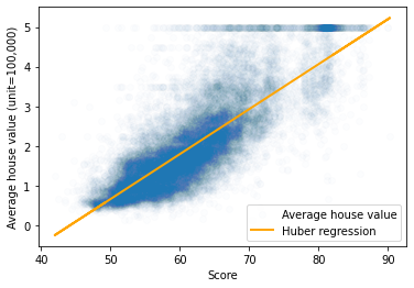
The following plot shows a perfect linear relationship between the score and average the house value.
[13]:
plt.scatter(score, y, alpha=0.01, label="Average house value")
plt.plot(score, y_pred, label="Huber regression", linewidth=2, color="orange")
plt.ylabel("Average house value (unit=100,000)")
plt.xlabel("Score")
plt.legend()
plt.show()