Tutorial: optimal binning with binary target under uncertainty¶

The drawback of performing optimal binning given only expected event rates is that variability of event rates in different periods is not taken into account. In this tutorial, we show how scenario-based stochastic programming allows incorporating uncertainty without much difficulty.

[1]:

import matplotlib.pyplot as plt
import numpy as np
import pandas as pd

from scipy import stats

[2]:

from optbinning import OptimalBinning
from optbinning.binning.uncertainty import SBOptimalBinning

Scenario generation¶

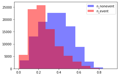
We generate three scenarios, all equally likely, aiming to represent three economic scenarios severity using the customer’s score variable, for instance.

Scenario 0 - Normal (Realistic): A low customer’ score has a higher event rate (default rate, churn, etc) than a high customer’s score. The population corresponding to non-event and event are reasonably separated.

[3]:

N0 = int(1e5)

xe = stats.beta(a=4, b=15).rvs(size=N0, random_state=42)
ye = stats.bernoulli(p=0.7).rvs(size=N0, random_state=42)
xn = stats.beta(a=6, b=8).rvs(size=N0, random_state=42)
yn = stats.bernoulli(p=0.2).rvs(size=N0, random_state=42)

x0 = np.concatenate((xn, xe), axis=0)
y0 = np.concatenate((yn, ye), axis=0)

[4]:

def plot_distribution(x, y):
    plt.hist(x[y == 0], label="n_nonevent", color="b", alpha=0.5)
    plt.hist(x[y == 1], label="n_event", color="r", alpha=0.5)
    plt.legend()
    plt.show()

[5]:

plot_distribution(x0, y0)

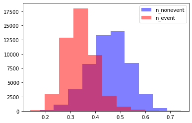
../_images/tutorials_tutorial_binary_under_uncertainty_9_0.png

Scenario 1: Good (Optimistic): A low customer’ score has a much higher event rate (default rate, churn, etc) than a high customer’s score. The population corresponding to non-event and event rate are very well separated, showing minimum overlap regions.

[6]:

N1 = int(5e4)

xe = stats.beta(a=25, b=50).rvs(size=N1, random_state=42)
ye = stats.bernoulli(p=0.9).rvs(size=N1, random_state=42)
xn = stats.beta(a=22, b=25).rvs(size=N1, random_state=42)
yn = stats.bernoulli(p=0.05).rvs(size=N1, random_state=42)

x1 = np.concatenate((xn, xe), axis=0)
y1 = np.concatenate((yn, ye), axis=0)

[7]:

plot_distribution(x1, y1)

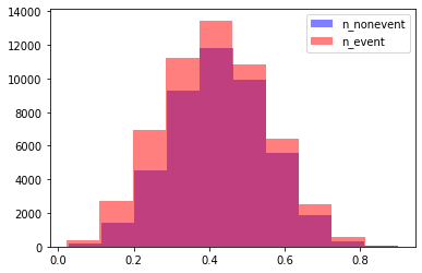
../_images/tutorials_tutorial_binary_under_uncertainty_12_0.png

Scenario 2: Bad (Pessimistic): Customer’s behavior cannot be accurately segmented, and a general increase in event rates is exhibited. The populations corresponding to non-event and event are practically overlapped.

[8]:

N2 = int(5e4)

xe = stats.beta(a=4, b=6).rvs(size=N2, random_state=42)
ye = stats.bernoulli(p=0.7).rvs(size=N2, random_state=42)
xn = stats.beta(a=8, b=10).rvs(size=N2, random_state=42)
yn = stats.bernoulli(p=0.4).rvs(size=N2, random_state=42)

x2 = np.concatenate((xn, xe), axis=0)
y2 = np.concatenate((yn, ye), axis=0)

[9]:

plot_distribution(x2, y2)

../_images/tutorials_tutorial_binary_under_uncertainty_15_0.png

Scenario-based stochastic optimal binning¶

Prepare scenarios data and instantiate an SBOptimalBinning object class. We set a descending monotonicity constraint with respect to event rate and a minimum bin size.

[10]:

X = [x0, x1, x2]
Y = [y0, y1, y2]

[11]:

sboptb = SBOptimalBinning(monotonic_trend="descending", min_bin_size=0.05)
sboptb.fit(X, Y)

[11]:

SBOptimalBinning(min_bin_size=0.05, monotonic_trend='descending')

[12]:

sboptb.status

[12]:

'OPTIMAL'

We obtain “only” three splits guaranteeing feasibility for each scenario.

[13]:

sboptb.splits

[13]:

array([0.28578988, 0.36384453, 0.43260857])

[14]:

sboptb.information(print_level=2)

optbinning (Version 0.19.0)
Copyright (c) 2019-2024 Guillermo Navas-Palencia, Apache License 2.0

  Begin options
    name                                       * d
    prebinning_method                   cart   * d
    max_n_prebins                         20   * d
    min_prebin_size                     0.05   * d
    min_n_bins                            no   * d
    max_n_bins                            no   * d
    min_bin_size                        0.05   * U
    max_bin_size                          no   * d
    monotonic_trend               descending   * U
    min_event_rate_diff                    0   * d
    max_pvalue                            no   * d
    max_pvalue_policy            consecutive   * d
    class_weight                          no   * d
    user_splits                           no   * d
    user_splits_fixed                     no   * d
    special_codes                         no   * d
    split_digits                          no   * d
    time_limit                           100   * d
    verbose                            False   * d
  End options

  Name    : UNKNOWN
  Status  : OPTIMAL

  Pre-binning statistics
    Number of pre-bins                    16
    Number of refinements                  1

  Solver statistics
    Type                                  cp
    Number of booleans                    40
    Number of branches                    91
    Number of conflicts                    1
    Objective value                  2736534
    Best objective bound             2736534

  Timing
    Total time                          1.21 sec
    Pre-processing                      0.01 sec   (  0.90%)
    Pre-binning                         0.70 sec   ( 58.18%)
    Solver                              0.49 sec   ( 40.72%)
      model generation                  0.44 sec   ( 90.22%)
      optimizer                         0.05 sec   (  9.78%)
    Post-processing                     0.00 sec   (  0.10%)

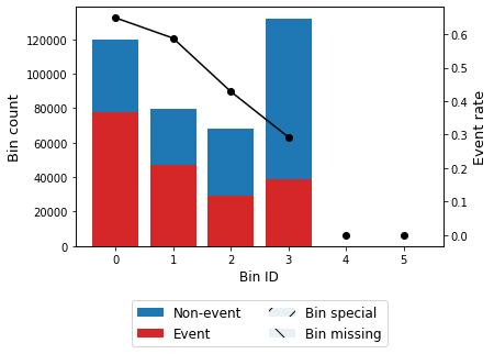
The binning table¶

As other optimal binning algorithms in OptBinning, SBOptimalBinning also returns a binning table displaying the binned data considering all scenarios.

[15]:

sboptb.binning_table.build()

[15]:

	Bin	Count	Count (%)	Non-event	Event	Event rate	WoE	IV	JS
0	(-inf, 0.29)	119678	0.299195	42005	77673	0.649017	-0.688603	0.138209	0.016943
1	[0.29, 0.36)	79729	0.199323	32837	46892	0.588142	-0.430175	0.036613	0.004542
2	[0.36, 0.43)	68378	0.170945	39045	29333	0.428983	0.212118	0.007633	0.000952
3	[0.43, inf)	132215	0.330537	93498	38717	0.292834	0.807778	0.201811	0.024562
4	Special	0	0.000000	0	0	0.000000	0.000000	0.000000	0.000000
5	Missing	0	0.000000	0	0	0.000000	0.000000	0.000000	0.000000
Totals		400000	1.000000	207385	192615	0.481538		0.384266	0.046999

[16]:

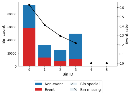
sboptb.binning_table.plot(metric="event_rate")

../_images/tutorials_tutorial_binary_under_uncertainty_27_0.png

[17]:

sboptb.binning_table.analysis()

---------------------------------------------
OptimalBinning: Binary Binning Table Analysis
---------------------------------------------

  General metrics

    Gini index               0.33117510
    IV (Jeffrey)             0.38426602
    JS (Jensen-Shannon)      0.04699884
    Hellinger                0.04750871
    Triangular               0.18408357
    KS                       0.28582022
    HHI                      0.26772434
    HHI (normalized)         0.12126921
    Cramer's V               0.30285954
    Quality score            0.87798527

  Monotonic trend            descending

  Significance tests

    Bin A  Bin B  t-statistic       p-value  P[A > B]     P[B > A]
        0      1   756.303469 1.709260e-166       1.0 1.110223e-16
        1      2  3732.973381  0.000000e+00       1.0 1.110223e-16
        2      3  3726.998391  0.000000e+00       1.0 1.110223e-16

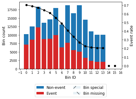
Expected value solution (EVS)¶

The expected value solution is calculated with the normal (expected) scenario.

[18]:

optb = OptimalBinning(monotonic_trend="descending", min_bin_size=0.05)
optb.fit(x0, y0)

[18]:

OptimalBinning(min_bin_size=0.05, monotonic_trend='descending')

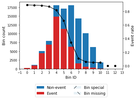
[19]:

optb.binning_table.build()

[19]:

	Bin	Count	Count (%)	Non-event	Event	Event rate	WoE	IV	JS
0	(-inf, 0.10)	10255	0.051275	3061	7194	0.701511	-1.054853	0.054945	0.006566
1	[0.10, 0.14)	12519	0.062595	3911	8608	0.687595	-0.989246	0.059422	0.007139
2	[0.14, 0.18)	18333	0.091665	6065	12268	0.669176	-0.904807	0.073418	0.008877
3	[0.18, 0.20)	13631	0.068155	4884	8747	0.641699	-0.783094	0.041320	0.005037
4	[0.20, 0.23)	14606	0.073030	5684	8922	0.610845	-0.651212	0.030891	0.003795
5	[0.23, 0.27)	17995	0.089975	8043	9952	0.553043	-0.413319	0.015470	0.001920
6	[0.27, 0.30)	13047	0.065235	6672	6375	0.488618	-0.154812	0.001572	0.000196
7	[0.30, 0.35)	18825	0.094125	11158	7667	0.407278	0.174884	0.002847	0.000355
8	[0.35, 0.39)	16401	0.082005	10903	5498	0.335223	0.484306	0.018430	0.002282
9	[0.39, 0.44)	18759	0.093795	13688	5071	0.270324	0.792634	0.053994	0.006578
10	[0.44, 0.49)	14549	0.072745	11273	3276	0.225170	1.035440	0.068446	0.008193
11	[0.49, 0.54)	11019	0.055095	8697	2322	0.210727	1.120202	0.059684	0.007093
12	[0.54, 0.60)	10030	0.050150	7957	2073	0.206680	1.144708	0.056454	0.006695
13	[0.60, inf)	10031	0.050155	7988	2043	0.203669	1.163174	0.058080	0.006877
14	Special	0	0.000000	0	0	0.000000	0.000000	0.000000	0.000000
15	Missing	0	0.000000	0	0	0.000000	0.000000	0.000000	0.000000
Totals		200000	1.000000	109984	90016	0.450080		0.594974	0.071603

[20]:

optb.binning_table.plot(metric="event_rate")

../_images/tutorials_tutorial_binary_under_uncertainty_33_0.png

[21]:

optb.binning_table.analysis()

---------------------------------------------
OptimalBinning: Binary Binning Table Analysis
---------------------------------------------

  General metrics

    Gini index               0.42141055
    IV (Jeffrey)             0.59497411
    JS (Jensen-Shannon)      0.07160267
    Hellinger                0.07295186
    Triangular               0.27638899
    KS                       0.34108533
    HHI                      0.07501900
    HHI (normalized)         0.01335360
    Cramer's V               0.36927482
    Quality score            0.16335319

  Monotonic trend            descending

  Significance tests

    Bin A  Bin B  t-statistic      p-value  P[A > B]     P[B > A]
        0      1     5.139745 2.338408e-02  0.988706 1.129409e-02
        1      2    11.534993 6.829832e-04  0.999721 2.787731e-04
        2      3    26.208899 3.064073e-07  1.000000 7.445353e-09
        3      4    28.661681 8.619251e-08  1.000000 4.436704e-09
        4      5   110.500800 7.611468e-26  1.000000 1.110223e-16
        5      6   125.906119 3.223792e-29  1.000000 1.110223e-16
        6      7   206.865709 6.632897e-47  1.000000 1.110223e-16
        7      8   194.419542 3.449032e-44  1.000000 1.110223e-16
        8      9   175.309976 5.122903e-40  1.000000 1.110223e-16
        9     10    88.957203 4.034468e-21  1.000000 1.110223e-16
       10     11     7.648694 5.681344e-03  0.997558 2.442113e-03
       11     12     0.520543 4.706103e-01  0.764881 2.351195e-01
       12     13     0.278879 5.974371e-01  0.701329 2.986709e-01

Scenario analysis¶

Scenario 0 - Normal (Realistic)¶

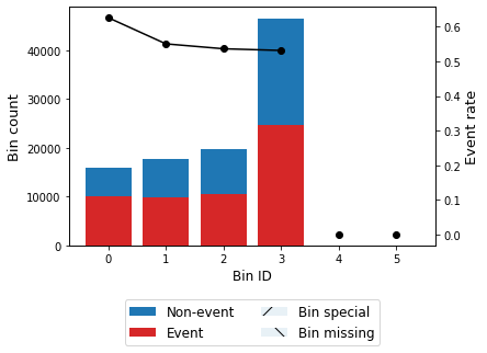
[22]:

bt0 = sboptb.binning_table_scenario(scenario_id=0)
bt0.build()

[22]:

	Bin	Count	Count (%)	Non-event	Event	Event rate	WoE	IV	JS
0	(-inf, 0.29)	93851	0.469255	34903	58948	0.628102	-0.724430	0.244506	0.029912
1	[0.29, 0.36)	32141	0.160705	18945	13196	0.410566	0.161279	0.004138	0.000517
2	[0.36, 0.43)	24488	0.122440	17289	7199	0.293981	0.675781	0.052184	0.006402
3	[0.43, inf)	49520	0.247600	38847	10673	0.215529	1.091566	0.256123	0.030515
4	Special	0	0.000000	0	0	0.000000	0.000000	0.000000	0.000000
5	Missing	0	0.000000	0	0	0.000000	0.000000	0.000000	0.000000
Totals		200000	1.000000	109984	90016	0.450080		0.556952	0.067345

[23]:

bt0.plot(metric="event_rate")

../_images/tutorials_tutorial_binary_under_uncertainty_38_0.png

[24]:

optb0 = OptimalBinning(monotonic_trend="descending", min_bin_size=0.05)
optb0.fit(x0, y0)

[24]:

OptimalBinning(min_bin_size=0.05, monotonic_trend='descending')

[25]:

optb0.binning_table.build()

[25]:

	Bin	Count	Count (%)	Non-event	Event	Event rate	WoE	IV	JS
0	(-inf, 0.10)	10255	0.051275	3061	7194	0.701511	-1.054853	0.054945	0.006566
1	[0.10, 0.14)	12519	0.062595	3911	8608	0.687595	-0.989246	0.059422	0.007139
2	[0.14, 0.18)	18333	0.091665	6065	12268	0.669176	-0.904807	0.073418	0.008877
3	[0.18, 0.20)	13631	0.068155	4884	8747	0.641699	-0.783094	0.041320	0.005037
4	[0.20, 0.23)	14606	0.073030	5684	8922	0.610845	-0.651212	0.030891	0.003795
5	[0.23, 0.27)	17995	0.089975	8043	9952	0.553043	-0.413319	0.015470	0.001920
6	[0.27, 0.30)	13047	0.065235	6672	6375	0.488618	-0.154812	0.001572	0.000196
7	[0.30, 0.35)	18825	0.094125	11158	7667	0.407278	0.174884	0.002847	0.000355
8	[0.35, 0.39)	16401	0.082005	10903	5498	0.335223	0.484306	0.018430	0.002282
9	[0.39, 0.44)	18759	0.093795	13688	5071	0.270324	0.792634	0.053994	0.006578
10	[0.44, 0.49)	14549	0.072745	11273	3276	0.225170	1.035440	0.068446	0.008193
11	[0.49, 0.54)	11019	0.055095	8697	2322	0.210727	1.120202	0.059684	0.007093
12	[0.54, 0.60)	10030	0.050150	7957	2073	0.206680	1.144708	0.056454	0.006695
13	[0.60, inf)	10031	0.050155	7988	2043	0.203669	1.163174	0.058080	0.006877
14	Special	0	0.000000	0	0	0.000000	0.000000	0.000000	0.000000
15	Missing	0	0.000000	0	0	0.000000	0.000000	0.000000	0.000000
Totals		200000	1.000000	109984	90016	0.450080		0.594974	0.071603

[26]:

optb0.binning_table.plot(metric="event_rate")

../_images/tutorials_tutorial_binary_under_uncertainty_41_0.png

Apply expected value solution to scenario 0.

[27]:

evs_optb0 = OptimalBinning(user_splits=optb.splits)
evs_optb0.fit(x0, y0)

[27]:

OptimalBinning(user_splits=array([0.1008646 , 0.13640077, 0.17635711, 0.20390539, 0.23334569,
       0.27135116, 0.30051835, 0.34623086, 0.38964605, 0.44464479,
       0.49356021, 0.53990114, 0.59801421]))

[28]:

evs_optb0.binning_table.build()

[28]:

	Bin	Count	Count (%)	Non-event	Event	Event rate	WoE	IV	JS
0	(-inf, 0.10)	10255	0.051275	3061	7194	0.701511	-1.054853	0.054945	0.006566
1	[0.10, 0.14)	12519	0.062595	3911	8608	0.687595	-0.989246	0.059422	0.007139
2	[0.14, 0.18)	18333	0.091665	6065	12268	0.669176	-0.904807	0.073418	0.008877
3	[0.18, 0.20)	13631	0.068155	4884	8747	0.641699	-0.783094	0.041320	0.005037
4	[0.20, 0.23)	14606	0.073030	5684	8922	0.610845	-0.651212	0.030891	0.003795
5	[0.23, 0.27)	17995	0.089975	8043	9952	0.553043	-0.413319	0.015470	0.001920
6	[0.27, 0.30)	13047	0.065235	6672	6375	0.488618	-0.154812	0.001572	0.000196
7	[0.30, 0.35)	18825	0.094125	11158	7667	0.407278	0.174884	0.002847	0.000355
8	[0.35, 0.39)	16401	0.082005	10903	5498	0.335223	0.484306	0.018430	0.002282
9	[0.39, 0.44)	18759	0.093795	13688	5071	0.270324	0.792634	0.053994	0.006578
10	[0.44, 0.49)	14549	0.072745	11273	3276	0.225170	1.035440	0.068446	0.008193
11	[0.49, 0.54)	11019	0.055095	8697	2322	0.210727	1.120202	0.059684	0.007093
12	[0.54, 0.60)	10030	0.050150	7957	2073	0.206680	1.144708	0.056454	0.006695
13	[0.60, inf)	10031	0.050155	7988	2043	0.203669	1.163174	0.058080	0.006877
14	Special	0	0.000000	0	0	0.000000	0.000000	0.000000	0.000000
15	Missing	0	0.000000	0	0	0.000000	0.000000	0.000000	0.000000
Totals		200000	1.000000	109984	90016	0.450080		0.594974	0.071603

[29]:

evs_optb0.binning_table.plot(metric="event_rate")

../_images/tutorials_tutorial_binary_under_uncertainty_45_0.png

The expected value solution applied to scenarion 0 does not satisfy the min_bin_size constraint, hence the solution is not feasible.

[30]:

EVS_0 = 0.594974

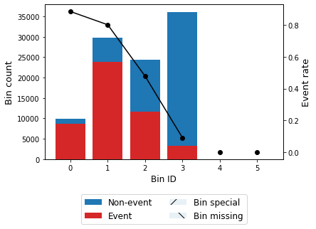
Scenario 1: Good (Optimistic)

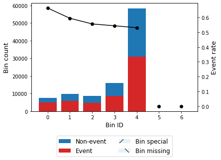
[31]:

bt1 = sboptb.binning_table_scenario(scenario_id=1)
bt1.build()

[31]:

	Bin	Count	Count (%)	Non-event	Event	Event rate	WoE	IV	JS
0	(-inf, 0.29)	9840	0.09840	1126	8714	0.885569	-2.146624	0.347828	0.036679
1	[0.29, 0.36)	29807	0.29807	5902	23905	0.801993	-1.499161	0.586072	0.067087
2	[0.36, 0.43)	24262	0.24262	12658	11604	0.478279	-0.013425	0.000044	0.000005
3	[0.43, inf)	36091	0.36091	32821	3270	0.090604	2.205914	1.226988	0.128301
4	Special	0	0.00000	0	0	0.000000	0.000000	0.000000	0.000000
5	Missing	0	0.00000	0	0	0.000000	0.000000	0.000000	0.000000
Totals		100000	1.00000	52507	47493	0.474930		2.160931	0.232072

[32]:

bt1.plot(metric="event_rate")

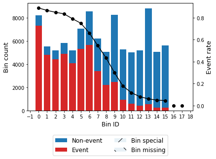
../_images/tutorials_tutorial_binary_under_uncertainty_50_0.png

[33]:

optb1 = OptimalBinning(monotonic_trend="descending", min_bin_size=0.05)
optb1.fit(x1, y1)

[33]:

OptimalBinning(min_bin_size=0.05, monotonic_trend='descending')

[34]:

optb1.binning_table.build()

[34]:

	Bin	Count	Count (%)	Non-event	Event	Event rate	WoE	IV	JS
0	(-inf, 0.28)	8209	0.08209	908	7301	0.889390	-2.184886	0.298095	0.031264
1	[0.28, 0.30)	5545	0.05545	738	4807	0.866907	-1.974249	0.172075	0.018581
2	[0.30, 0.31)	5186	0.05186	777	4409	0.850174	-1.836327	0.143301	0.015756
3	[0.31, 0.33)	5837	0.05837	956	4881	0.836217	-1.730712	0.146359	0.016307
4	[0.33, 0.34)	5176	0.05176	1077	4099	0.791924	-1.436928	0.094544	0.010896
5	[0.34, 0.36)	7055	0.07055	1760	5295	0.750532	-1.201813	0.093706	0.011056
6	[0.36, 0.38)	8537	0.08537	2882	5655	0.662411	-0.774420	0.049704	0.006062
7	[0.38, 0.40)	6189	0.06189	2802	3387	0.547261	-0.289975	0.005205	0.000648
8	[0.40, 0.41)	5058	0.05058	2862	2196	0.434164	0.164519	0.001360	0.000170
9	[0.41, 0.44)	8246	0.08246	5781	2465	0.298933	0.752021	0.043766	0.005345
10	[0.44, 0.45)	5253	0.05253	4321	932	0.177422	1.433545	0.089840	0.010358
11	[0.45, 0.47)	5009	0.05009	4420	589	0.117588	1.915105	0.137461	0.014960
12	[0.47, 0.49)	5204	0.05204	4780	424	0.081476	2.322098	0.190662	0.019603
13	[0.49, 0.53)	8825	0.08825	8283	542	0.061416	2.626330	0.384332	0.037733
14	[0.53, 0.56)	5061	0.05061	4807	254	0.050188	2.840130	0.244824	0.023237
15	[0.56, inf)	5610	0.05610	5353	257	0.045811	2.935972	0.283430	0.026488
16	Special	0	0.00000	0	0	0.000000	0.000000	0.000000	0.000000
17	Missing	0	0.00000	0	0	0.000000	0.000000	0.000000	0.000000
Totals		100000	1.00000	52507	47493	0.474930		2.378665	0.248465

[35]:

optb1.binning_table.plot(metric="event_rate")

../_images/tutorials_tutorial_binary_under_uncertainty_53_0.png

Apply expected value solution to scenario 1.

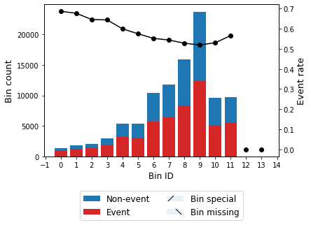
[36]:

evs_optb1 = OptimalBinning(user_splits=optb.splits)
evs_optb1.fit(x1, y1)

[36]:

OptimalBinning(user_splits=array([0.1008646 , 0.13640077, 0.17635711, 0.20390539, 0.23334569,
       0.27135116, 0.30051835, 0.34623086, 0.38964605, 0.44464479,
       0.49356021, 0.53990114, 0.59801421]))

[37]:

evs_optb1.binning_table.build()

[37]:

	Bin	Count	Count (%)	Non-event	Event	Event rate	WoE	IV	JS
0	(-inf, 0.20)	247	0.00247	26	221	0.894737	-2.240430	0.009316	0.000969
1	[0.20, 0.23)	1092	0.01092	118	974	0.891941	-2.211091	0.040377	0.004219
2	[0.23, 0.27)	5037	0.05037	566	4471	0.887632	-2.167137	0.180654	0.018995
3	[0.27, 0.30)	7918	0.07918	1019	6899	0.871306	-2.012919	0.253339	0.027214
4	[0.30, 0.35)	18126	0.18126	3313	14813	0.817224	-1.598015	0.397590	0.045005
5	[0.35, 0.39)	17091	0.17091	5742	11349	0.664034	-0.781686	0.101310	0.012351
6	[0.39, 0.44)	18095	0.18095	11857	6238	0.344736	0.541895	0.051194	0.006322
7	[0.44, 0.49)	14295	0.14295	12739	1556	0.108849	2.002186	0.420164	0.045199
8	[0.49, 0.54)	10111	0.10111	9523	588	0.058154	2.684374	0.453620	0.044133
9	[0.54, 0.60)	6215	0.06215	5918	297	0.047788	2.891658	0.307832	0.028976
10	[0.60, inf)	1773	0.01773	1686	87	0.049069	2.863842	0.086712	0.008199
11	Special	0	0.00000	0	0	0.000000	0.000000	0.000000	0.000000
12	Missing	0	0.00000	0	0	0.000000	0.000000	0.000000	0.000000
Totals		100000	1.00000	52507	47493	0.474930		2.302108	0.241582

[38]:

evs_optb1.binning_table.plot(metric="event_rate")

../_images/tutorials_tutorial_binary_under_uncertainty_57_0.png

[39]:

evs_optb1.binning_table.analysis()

---------------------------------------------
OptimalBinning: Binary Binning Table Analysis
---------------------------------------------

  General metrics

    Gini index               0.72566718
    IV (Jeffrey)             2.30210757
    JS (Jensen-Shannon)      0.24158211
    Hellinger                0.26182242
    Triangular               0.84830395
    KS                       0.61004329
    HHI                      0.13857518
    HHI (normalized)         0.06678978
    Cramer's V               0.64902999
    Quality score            0.00000000

  Monotonic trend                valley

  Significance tests

    Bin A  Bin B  t-statistic       p-value  P[A > B]     P[B > A]
        0      1     0.016401  8.980961e-01  0.566231 4.337689e-01
        1      2     0.168135  6.817748e-01  0.666387 3.336129e-01
        2      3     7.641448  5.704212e-03  0.997457 2.543322e-03
        3      4   116.236493  4.218674e-27  1.000000 1.110223e-16
        4      5  1080.747496 5.050568e-237  1.000000 1.110223e-16
        5      6  3584.325798  0.000000e+00  1.000000 1.110223e-16
        6      7  2431.847481  0.000000e+00  1.000000 1.110223e-16
        7      8   189.938108  3.279750e-43  1.000000 1.110223e-16
        8      9     8.068486  4.504174e-03  0.998346 1.654368e-03
        9     10     0.049526  8.238907e-01  0.420232 5.797684e-01

The expected value solution applied to scenario 1 satisfies neither the min_bin_size constraint nor the monotonicity constraint, hence the solution is not feasible.

[40]:

EVS_1 = -np.inf

Scenario 2: Bad (Pessimistic)

[41]:

bt2 = sboptb.binning_table_scenario(scenario_id=2)
bt2.build()

[41]:

	Bin	Count	Count (%)	Non-event	Event	Event rate	WoE	IV	JS
0	(-inf, 0.29)	15987	0.15987	5976	10011	0.626196	-0.310979	1.509941e-02	1.879858e-03
1	[0.29, 0.36)	17781	0.17781	7990	9791	0.550644	0.001682	5.028570e-07	6.285711e-08
2	[0.36, 0.43)	19628	0.19628	9098	10530	0.536479	0.058781	6.800268e-04	8.499112e-05
3	[0.43, inf)	46604	0.46604	21830	24774	0.531585	0.078445	2.877876e-03	3.596423e-04
4	Special	0	0.00000	0	0	0.000000	0.000000	0.000000e+00	0.000000e+00
5	Missing	0	0.00000	0	0	0.000000	0.000000	0.000000e+00	0.000000e+00
Totals		100000	1.00000	44894	55106	0.551060		1.865782e-02	2.324554e-03

[42]:

bt2.plot(metric="event_rate")

../_images/tutorials_tutorial_binary_under_uncertainty_63_0.png

[43]:

optb2 = OptimalBinning(monotonic_trend="descending", min_bin_size=0.05)
optb2.fit(x2, y2)

[43]:

OptimalBinning(min_bin_size=0.05, monotonic_trend='descending')

[44]:

optb2.binning_table.build()

[44]:

	Bin	Count	Count (%)	Non-event	Event	Event rate	WoE	IV	JS
0	(-inf, 0.23)	7556	0.07556	2543	5013	0.663446	-0.473736	0.016261	0.002014
1	[0.23, 0.29)	9657	0.09657	3918	5739	0.594284	-0.176749	0.002982	0.000372
2	[0.29, 0.33)	8559	0.08559	3801	4758	0.555906	-0.019609	0.000033	0.000004
3	[0.33, 0.39)	15848	0.15848	7234	8614	0.543539	0.030358	0.000146	0.000018
4	[0.39, inf)	58380	0.58380	27398	30982	0.530695	0.082018	0.003941	0.000493
5	Special	0	0.00000	0	0	0.000000	0.000000	0.000000	0.000000
6	Missing	0	0.00000	0	0	0.000000	0.000000	0.000000	0.000000
Totals		100000	1.00000	44894	55106	0.551060		0.023364	0.002901

[45]:

optb2.binning_table.plot(metric="event_rate")

../_images/tutorials_tutorial_binary_under_uncertainty_66_0.png

Apply expected value solution to scenario 2.

[46]:

evs_optb2 = OptimalBinning(user_splits=optb.splits)
evs_optb2.fit(x2, y2)

[46]:

OptimalBinning(user_splits=array([0.1008646 , 0.13640077, 0.17635711, 0.20390539, 0.23334569,
       0.27135116, 0.30051835, 0.34623086, 0.38964605, 0.44464479,
       0.49356021, 0.53990114, 0.59801421]))

[47]:

evs_optb2.binning_table.build()

[47]:

	Bin	Count	Count (%)	Non-event	Event	Event rate	WoE	IV	JS
0	(-inf, 0.14)	1292	0.01292	405	887	0.686533	-0.579003	0.004096	5.050214e-04
1	[0.14, 0.18)	1850	0.01850	598	1252	0.676757	-0.533952	0.005019	6.200181e-04
2	[0.18, 0.20)	2002	0.02002	709	1293	0.645854	-0.395910	0.003037	3.771741e-04
3	[0.20, 0.23)	2944	0.02944	1049	1895	0.643682	-0.386427	0.004259	5.291176e-04
4	[0.23, 0.27)	5326	0.05326	2134	3192	0.599324	-0.197695	0.002054	2.563524e-04
5	[0.27, 0.30)	5390	0.05390	2291	3099	0.574954	-0.097137	0.000506	6.318381e-05
6	[0.30, 0.35)	10414	0.10414	4667	5747	0.551853	-0.003207	0.000001	1.338664e-07
7	[0.35, 0.39)	11782	0.11782	5375	6407	0.543796	0.029322	0.000101	1.267992e-05
8	[0.39, 0.44)	15901	0.15901	7509	8392	0.527766	0.093778	0.001404	1.754450e-04
9	[0.44, 0.54)	23757	0.23757	11416	12341	0.519468	0.127043	0.003854	4.814509e-04
10	[0.54, 0.60)	9639	0.09639	4529	5110	0.530138	0.084256	0.000687	8.582857e-05
11	[0.60, inf)	9703	0.09703	4212	5491	0.565907	-0.060218	0.000351	4.382723e-05
12	Special	0	0.00000	0	0	0.000000	0.000000	0.000000	0.000000e+00
13	Missing	0	0.00000	0	0	0.000000	0.000000	0.000000	0.000000e+00
Totals		100000	1.00000	44894	55106	0.551060		0.025370	3.150233e-03

[48]:

evs_optb2.binning_table.plot(metric="event_rate")

../_images/tutorials_tutorial_binary_under_uncertainty_70_0.png

[49]:

evs_optb2.binning_table.analysis()

---------------------------------------------
OptimalBinning: Binary Binning Table Analysis
---------------------------------------------

  General metrics

    Gini index               0.07657686
    IV (Jeffrey)             0.02536981
    JS (Jensen-Shannon)      0.00315023
    Hellinger                0.00316066
    Triangular               0.01251904
    KS                       0.05109803
    HHI                      0.13267476
    HHI (normalized)         0.06595743
    Cramer's V               0.07812501
    Quality score            0.00318975

  Monotonic trend                valley

  Significance tests

    Bin A  Bin B  t-statistic      p-value     P[A > B]  P[B > A]
        0      1     0.334525 5.630065e-01 7.193040e-01  0.280696
        1      2     4.095897 4.298741e-02 9.789856e-01  0.021014
        2      3     0.024540 8.755193e-01 5.627139e-01  0.437286
        3      4    15.757594 7.199834e-05 9.999743e-01  0.000026
        4      5     6.563219 1.041079e-02 9.951398e-01  0.004860
        5      6     7.690930 5.549902e-03 9.973851e-01  0.002615
        6      7     1.448735 2.287310e-01 8.858561e-01  0.114144
        7      8     6.989473 8.199050e-03 9.961485e-01  0.003852
        8      9     2.628779 1.049424e-01 9.478637e-01  0.052136
        9     10     3.128995 7.691114e-02 3.817921e-02  0.961821
       10     11    24.977930 5.799032e-07 4.353127e-08  1.000000

The expected value solution applied to scenario 2 satisfies neither the min_bin_size constraint nor the monotonicity constraint, hence the solution is not feasible.

[50]:

EVS_2 = -np.inf

Expected value of perfect information (EVPI)¶

If we have prior information about the incoming economic scenarios, we could take optimal solutions for each scenario, with total IV:

[51]:

DIV0 = optb0.binning_table.iv
DIV1 = optb1.binning_table.iv
DIV2 = optb2.binning_table.iv
DIV = (DIV0 + DIV1 + DIV2) / 3

[52]:

DIV

[52]:

0.9990011753826167

However, this information is unlikely to be available in advance, so the best we can do in the long run is to use the stochastic programming, with expected total IV:

[53]:

SIV = sboptb.binning_table.iv

[54]:

SIV

[54]:

0.38426601503532376

The difference, in the case of perfect information, is the expected value of perfect information (EVPI) given by:

[55]:

EVPI = DIV - SIV
EVPI

[55]:

0.6147351603472929

Value of stochastic solution (VSS)¶

The loss in IV by not considering stochasticity is the difference between the application of the expected value solution for each scenario and the stochastic model IV. The application of the EVS to each scenario results in infeasible solutions, thus

[56]:

VSS = SIV - (EVS_0 + EVS_1 + EVS_2)
VSS

[56]:

inf