Tutorial: optimal binning with multiclass target
Basic
To get us started, let’s load a well-known dataset from the UCI repository and transform the data into a pandas.DataFrame.
[1]:
import pandas as pd
from sklearn.datasets import load_wine
[2]:
data = load_wine()
df = pd.DataFrame(data.data, columns=data.feature_names)
We choose a variable to discretize and the multiclass target.
[3]:
variable = "ash"
x = df[variable].values
y = data.target
Import and instantiate an MulticlassOptimalBinning object class. We pass the variable name and a solver, in this case, we choose the constraint programming solver.
[4]:
from optbinning import MulticlassOptimalBinning
[5]:
optb = MulticlassOptimalBinning(name=variable, solver="cp")
We fit the optimal binning object with arrays x and y.
[6]:
optb.fit(x, y)
[6]:
MulticlassOptimalBinning(name='ash')In a Jupyter environment, please rerun this cell to show the HTML representation or trust the notebook.
On GitHub, the HTML representation is unable to render, please try loading this page with nbviewer.org.
Parameters
| name | 'ash' | |
| prebinning_method | 'cart' | |
| solver | 'cp' | |
| max_n_prebins | 20 | |
| min_prebin_size | 0.05 | |
| min_n_bins | None | |
| max_n_bins | None | |
| min_bin_size | None | |
| max_bin_size | None | |
| monotonic_trend | 'auto' | |
| min_event_rate_diff | 0 | |
| max_pvalue | None | |
| max_pvalue_policy | 'consecutive' | |
| outlier_detector | None | |
| outlier_params | None | |
| user_splits | None | |
| user_splits_fixed | None | |
| special_codes | None | |
| split_digits | None | |
| mip_solver | 'bop' | |
| time_limit | 100 | |
| verbose | False |
You can check if an optimal solution has been found via the status attribute:
[7]:
optb.status
[7]:
'OPTIMAL'
You can also retrieve the optimal split points via the splits attribute:
[8]:
optb.splits
[8]:
array([2.1450001 , 2.245 , 2.31499994, 2.6049999 , 2.6450001 ])
The binning table
The optimal binning algorithms return a binning table; a binning table displays the binned data and several metrics for each bin. Class OptimalBinning returns an object MulticlassBinningTable via the binning_table attribute.
[9]:
binning_table = optb.binning_table
[10]:
type(binning_table)
[10]:
optbinning.binning.binning_statistics.MulticlassBinningTable
The binning_table is instantiated, but not built. Therefore, the first step is to call the method build, which returns a pandas.DataFrame.
[11]:
binning_table.build()
[11]:
| Bin | Count | Count (%) | Event_0 | Event_1 | Event_2 | Event_rate_0 | Event_rate_1 | Event_rate_2 | |
|---|---|---|---|---|---|---|---|---|---|
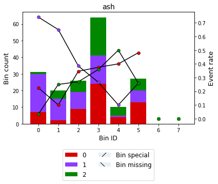
| 0 | (-inf, 2.15) | 31 | 0.174157 | 7 | 23 | 1 | 0.225806 | 0.741935 | 0.032258 |
| 1 | [2.15, 2.25) | 20 | 0.112360 | 2 | 13 | 5 | 0.100000 | 0.650000 | 0.250000 |
| 2 | [2.25, 2.31) | 26 | 0.146067 | 9 | 10 | 7 | 0.346154 | 0.384615 | 0.269231 |
| 3 | [2.31, 2.60) | 64 | 0.359551 | 24 | 17 | 23 | 0.375000 | 0.265625 | 0.359375 |
| 4 | [2.60, 2.65) | 10 | 0.056180 | 4 | 1 | 5 | 0.400000 | 0.100000 | 0.500000 |
| 5 | [2.65, inf) | 27 | 0.151685 | 13 | 7 | 7 | 0.481481 | 0.259259 | 0.259259 |
| 6 | Special | 0 | 0.000000 | 0 | 0 | 0 | 0.000000 | 0.000000 | 0.000000 |
| 7 | Missing | 0 | 0.000000 | 0 | 0 | 0 | 0.000000 | 0.000000 | 0.000000 |
| Totals | 178 | 1.000000 | 59 | 71 | 48 | 0.331461 | 0.398876 | 0.269663 |
Let’s describe the columns of this binning table:
Bin: the intervals delimited by the optimal split points.
Count: the number of records for each bin.
Count (%): the percentage of records for each bin.
Event: the number of event records \((y = class)\) for each bin.
Event rate: the percentage of event records for each bin. This is computed using one-vs-all or one-vs-rest approach.
The last row shows the total number of records, event records, and event rates.
You can use the method plot to visualize the histogram and event rate curve. Note that the Bin ID corresponds to the binning table index.
[12]:
binning_table.plot()
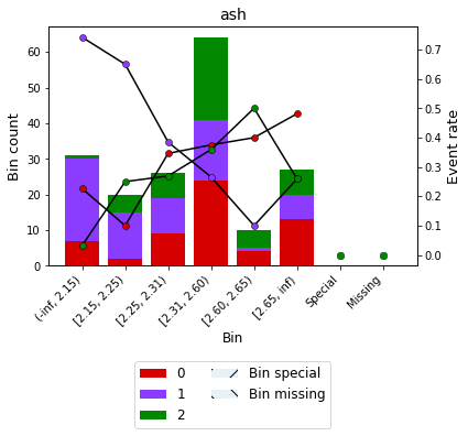
Alternatively, the Bin can be visualized using show_bin_labels=True (since version 0.15.1)
[13]:
binning_table.plot(show_bin_labels=True)
Transformation
Now that we have checked the binned data, we can transform our original data into a measure based on the one-vs-rest WoE metric. You can check the correctness of the transformation using pandas value_counts method, for instance.
[14]:
x_transform_woe = optb.transform(x, metric="bins")
[15]:
pd.Series(x_transform_woe).value_counts()
[15]:
[2.31, 2.60)    64
(-inf, 2.15)    31
[2.65, inf)     27
[2.25, 2.31)    26
[2.15, 2.25)    20
[2.60, 2.65)    10
Name: count, dtype: int64
Advanced
Many of the advanced options have been covered in the previous tutorials with a binary target. Check it out! In this section, we focus on the binning table statistical analysis and the event rate monotonicity trends.
Binning table statistical analysis
The analysis method performs a statistical analysis of the binning table, computing the Jensen-shannon divergence and the quality score. Additionally, a statistical significance test between consecutive bins of the contingency table is performed using the Chi-square test.
[16]:
binning_table.analysis()
-------------------------------------------------
OptimalBinning: Multiclass Binning Table Analysis
-------------------------------------------------

  General metrics

    JS (Jensen-Shannon)      0.10989515
    HHI                      0.21973236
    HHI (normalized)         0.06367883
    Cramer's V               0.31694075
    Quality score            0.05543813

  Monotonic trend

    Class  0                     valley
    Class  1                     valley
    Class  2                       peak

  Significance tests

    Bin A  Bin B  t-statistic  p-value
        0      1     6.135081 0.046535
        1      2     4.472669 0.106849
        2      3     1.365275 0.505282
        3      4     1.441642 0.486353
        4      5     2.265477 0.322150
Event rate monotonicity
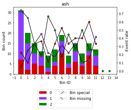
The monotonic_trend option permits forcing a monotonic trend to the event rate curve of each class. The default setting “auto” should be the preferred option, however, some business constraints might require to impose different trends. The default setting “auto” chooses the monotonic trend most likely to maximize the information value from the options “ascending”, “descending”, “peak” and “valley” for each class using a machine-learning-based classifier.
A good starting point to decide which monotonic trend to enforce for each class is to use monotonic_trend=None.
[17]:
optb = MulticlassOptimalBinning(name=variable, solver="mip", monotonic_trend=None)

optb.fit(x, y)
[17]:
MulticlassOptimalBinning(monotonic_trend=None, name='ash', solver='mip')In a Jupyter environment, please rerun this cell to show the HTML representation or trust the notebook.
On GitHub, the HTML representation is unable to render, please try loading this page with nbviewer.org.
Parameters
| name | 'ash' | |
| solver | 'mip' | |
| monotonic_trend | None | |
| prebinning_method | 'cart' | |
| max_n_prebins | 20 | |
| min_prebin_size | 0.05 | |
| min_n_bins | None | |
| max_n_bins | None | |
| min_bin_size | None | |
| max_bin_size | None | |
| min_event_rate_diff | 0 | |
| max_pvalue | None | |
| max_pvalue_policy | 'consecutive' | |
| outlier_detector | None | |
| outlier_params | None | |
| user_splits | None | |
| user_splits_fixed | None | |
| special_codes | None | |
| split_digits | None | |
| mip_solver | 'bop' | |
| time_limit | 100 | |
| verbose | False |
[18]:
binning_table = optb.binning_table
binning_table.build()
[18]:
| Bin | Count | Count (%) | Event_0 | Event_1 | Event_2 | Event_rate_0 | Event_rate_1 | Event_rate_2 | |
|---|---|---|---|---|---|---|---|---|---|
| 0 | (-inf, 2.15) | 31 | 0.174157 | 7 | 23 | 1 | 0.225806 | 0.741935 | 0.032258 |
| 1 | [2.15, 2.25) | 20 | 0.112360 | 2 | 13 | 5 | 0.100000 | 0.650000 | 0.250000 |
| 2 | [2.25, 2.28) | 15 | 0.084270 | 5 | 5 | 5 | 0.333333 | 0.333333 | 0.333333 |
| 3 | [2.28, 2.31) | 11 | 0.061798 | 4 | 5 | 2 | 0.363636 | 0.454545 | 0.181818 |
| 4 | [2.31, 2.35) | 9 | 0.050562 | 1 | 2 | 6 | 0.111111 | 0.222222 | 0.666667 |
| 5 | [2.35, 2.39) | 12 | 0.067416 | 4 | 2 | 6 | 0.333333 | 0.166667 | 0.500000 |
| 6 | [2.39, 2.47) | 19 | 0.106742 | 10 | 6 | 3 | 0.526316 | 0.315789 | 0.157895 |
| 7 | [2.47, 2.50) | 9 | 0.050562 | 3 | 2 | 4 | 0.333333 | 0.222222 | 0.444444 |
| 8 | [2.50, 2.60) | 15 | 0.084270 | 6 | 5 | 4 | 0.400000 | 0.333333 | 0.266667 |
| 9 | [2.60, 2.65) | 10 | 0.056180 | 4 | 1 | 5 | 0.400000 | 0.100000 | 0.500000 |
| 10 | [2.65, 2.73) | 15 | 0.084270 | 9 | 2 | 4 | 0.600000 | 0.133333 | 0.266667 |
| 11 | [2.73, inf) | 12 | 0.067416 | 4 | 5 | 3 | 0.333333 | 0.416667 | 0.250000 |
| 12 | Special | 0 | 0.000000 | 0 | 0 | 0 | 0.000000 | 0.000000 | 0.000000 |
| 13 | Missing | 0 | 0.000000 | 0 | 0 | 0 | 0.000000 | 0.000000 | 0.000000 |
| Totals | 178 | 1.000000 | 59 | 71 | 48 | 0.331461 | 0.398876 | 0.269663 |
[19]:
binning_table.plot()
[20]:
binning_table.analysis()
-------------------------------------------------
OptimalBinning: Multiclass Binning Table Analysis
-------------------------------------------------

  General metrics

    JS (Jensen-Shannon)      0.15199204
    HHI                      0.09683121
    HHI (normalized)         0.01472495
    Cramer's V               0.37833165
    Quality score            0.00408300

  Monotonic trend

    Class  0               no monotonic
    Class  1               no monotonic
    Class  2               no monotonic

  Significance tests

    Bin A  Bin B  t-statistic  p-value
        0      1     6.135081 0.046535
        1      2     4.212963 0.121665
        2      3     0.800385 0.670191
        3      4     4.935065 0.084794
        4      5     1.400000 0.496585
        5      6     4.205201 0.122138
        6      7     2.682861 0.261471
        7      8     0.838095 0.657673
        8      9     2.268519 0.321660
        9     10     1.424501 0.490539
       10     11     3.056044 0.216964
For example, we can decide that we do not care about class 2 and only force classes 0 and 1.
[21]:
optb = MulticlassOptimalBinning(name=variable, solver="mip",
                                monotonic_trend=["ascending", "auto", None],
                                verbose=True)

optb.fit(x, y)
2026-09-12 18:20:19,999 | INFO : Optimal binning started.
2026-09-12 18:20:20,003 | INFO : Options: check parameters.
2026-09-12 18:20:20,005 | INFO : Pre-processing started.
2026-09-12 18:20:20,011 | INFO : Pre-processing: number of samples: 178
2026-09-12 18:20:20,015 | INFO : Pre-processing: number of clean samples: 178
2026-09-12 18:20:20,017 | INFO : Pre-processing: number of missing samples: 0
2026-09-12 18:20:20,019 | INFO : Pre-processing: number of special samples: 0
2026-09-12 18:20:20,021 | INFO : Pre-processing terminated. Time: 0.0003s
2026-09-12 18:20:20,024 | INFO : Pre-binning started.
2026-09-12 18:20:20,031 | INFO : Pre-binning: number prebins removed: 1
2026-09-12 18:20:20,033 | INFO : Pre-binning: number of prebins: 12
2026-09-12 18:20:20,036 | INFO : Pre-binning: number of refinements: 1
2026-09-12 18:20:20,038 | INFO : Pre-binning terminated. Time: 0.0081s
2026-09-12 18:20:20,041 | INFO : Optimizer started.
2026-09-12 18:20:20,047 | INFO : Optimizer: classifier predicts valley monotonic trend.
2026-09-12 18:20:20,048 | INFO : Optimizer: build model...
2026-09-12 18:20:20,183 | INFO : Optimizer: solve...
2026-09-12 18:20:20,191 | INFO : Optimizer terminated. Time: 0.1486s
2026-09-12 18:20:20,194 | INFO : Post-processing started.
2026-09-12 18:20:20,196 | INFO : Post-processing: compute binning information.
2026-09-12 18:20:20,200 | INFO : Post-processing terminated. Time: 0.0001s
2026-09-12 18:20:20,201 | INFO : Optimal binning terminated. Status: OPTIMAL. Time: 0.2029s
[21]:
MulticlassOptimalBinning(monotonic_trend=['ascending', 'auto', None],
                         name='ash', solver='mip', verbose=True)
In a Jupyter environment, please rerun this cell to show the HTML representation or trust the notebook. On GitHub, the HTML representation is unable to render, please try loading this page with nbviewer.org.
Parameters
| name | 'ash' | |
| solver | 'mip' | |
| monotonic_trend | ['ascending', 'auto', ...] | |
| verbose | True | |
| prebinning_method | 'cart' | |
| max_n_prebins | 20 | |
| min_prebin_size | 0.05 | |
| min_n_bins | None | |
| max_n_bins | None | |
| min_bin_size | None | |
| max_bin_size | None | |
| min_event_rate_diff | 0 | |
| max_pvalue | None | |
| max_pvalue_policy | 'consecutive' | |
| outlier_detector | None | |
| outlier_params | None | |
| user_splits | None | |
| user_splits_fixed | None | |
| special_codes | None | |
| split_digits | None | |
| mip_solver | 'bop' | |
| time_limit | 100 |
[22]:
binning_table = optb.binning_table
binning_table.build()
[22]:
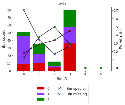
| Bin | Count | Count (%) | Event_0 | Event_1 | Event_2 | Event_rate_0 | Event_rate_1 | Event_rate_2 | |
|---|---|---|---|---|---|---|---|---|---|
| 0 | (-inf, 2.25) | 51 | 0.286517 | 9 | 36 | 6 | 0.176471 | 0.705882 | 0.117647 |
| 1 | [2.25, 2.35) | 35 | 0.196629 | 10 | 12 | 13 | 0.285714 | 0.342857 | 0.371429 |
| 2 | [2.35, 2.39) | 12 | 0.067416 | 4 | 2 | 6 | 0.333333 | 0.166667 | 0.500000 |
| 3 | [2.39, inf) | 80 | 0.449438 | 36 | 21 | 23 | 0.450000 | 0.262500 | 0.287500 |
| 4 | Special | 0 | 0.000000 | 0 | 0 | 0 | 0.000000 | 0.000000 | 0.000000 |
| 5 | Missing | 0 | 0.000000 | 0 | 0 | 0 | 0.000000 | 0.000000 | 0.000000 |
| Totals | 178 | 1.000000 | 59 | 71 | 48 | 0.331461 | 0.398876 | 0.269663 |
[23]:
binning_table.plot()
[24]:
binning_table.analysis()
-------------------------------------------------
OptimalBinning: Multiclass Binning Table Analysis
-------------------------------------------------

  General metrics

    JS (Jensen-Shannon)      0.08899633
    HHI                      0.32729453
    HHI (normalized)         0.10305938
    Cramer's V               0.30518651
    Quality score            0.09769235

  Monotonic trend

    Class  0                  ascending
    Class  1            valley (convex)
    Class  2             peak (concave)

  Significance tests

    Bin A  Bin B  t-statistic  p-value
        0      1    12.072711 0.002390
        1      2     1.364733 0.505419
        2      3     2.204828 0.332069
Event rate minimum difference
Since version 0.17.0, the parameter min_event_rate_diff is available for multiclass binning.
[25]:
optb = MulticlassOptimalBinning(name=variable, solver="mip",
                                monotonic_trend=None,
                                min_event_rate_diff=0.03)

optb.fit(x, y)
[25]:
MulticlassOptimalBinning(min_event_rate_diff=0.03, monotonic_trend=None,
                         name='ash', solver='mip')
In a Jupyter environment, please rerun this cell to show the HTML representation or trust the notebook. On GitHub, the HTML representation is unable to render, please try loading this page with nbviewer.org.
Parameters
| name | 'ash' | |
| solver | 'mip' | |
| monotonic_trend | None | |
| min_event_rate_diff | 0.03 | |
| prebinning_method | 'cart' | |
| max_n_prebins | 20 | |
| min_prebin_size | 0.05 | |
| min_n_bins | None | |
| max_n_bins | None | |
| min_bin_size | None | |
| max_bin_size | None | |
| max_pvalue | None | |
| max_pvalue_policy | 'consecutive' | |
| outlier_detector | None | |
| outlier_params | None | |
| user_splits | None | |
| user_splits_fixed | None | |
| special_codes | None | |
| split_digits | None | |
| mip_solver | 'bop' | |
| time_limit | 100 | |
| verbose | False |
[26]:
optb.information(print_level=2)
optbinning (Version 1.0.0)
Copyright (c) 2019-2026 Guillermo Navas-Palencia, Apache License 2.0

  Begin options
    name                                 ash   * U
    prebinning_method                   cart   * d
    solver                               mip   * U
    max_n_prebins                         20   * d
    min_prebin_size                     0.05   * d
    min_n_bins                            no   * d
    max_n_bins                            no   * d
    min_bin_size                          no   * d
    max_bin_size                          no   * d
    monotonic_trend                       no   * U
    min_event_rate_diff                 0.03   * U
    max_pvalue                            no   * d
    max_pvalue_policy            consecutive   * d
    user_splits                           no   * d
    user_splits_fixed                     no   * d
    special_codes                         no   * d
    split_digits                          no   * d
    mip_solver                           bop   * d
    time_limit                           100   * d
    verbose                            False   * d
  End options

  Name    : ash
  Status  : OPTIMAL

  Pre-binning statistics
    Number of pre-bins                    12
    Number of refinements                  1

  Solver statistics
    Type                                 mip
    Number of variables                  196
    Number of constraints                 78
    Objective value                   2.2657
    Best objective bound              2.2657

  Timing
    Total time                          0.05 sec
    Pre-processing                      0.00 sec   (  0.61%)
    Pre-binning                         0.01 sec   ( 11.76%)
    Solver                              0.04 sec   ( 85.90%)
    Post-processing                     0.00 sec   (  0.63%)
[27]:
binning_table = optb.binning_table
binning_table.build()
[27]:
| Bin | Count | Count (%) | Event_0 | Event_1 | Event_2 | Event_rate_0 | Event_rate_1 | Event_rate_2 | |
|---|---|---|---|---|---|---|---|---|---|
| 0 | (-inf, 2.15) | 31 | 0.174157 | 7 | 23 | 1 | 0.225806 | 0.741935 | 0.032258 |
| 1 | [2.15, 2.25) | 20 | 0.112360 | 2 | 13 | 5 | 0.100000 | 0.650000 | 0.250000 |
| 2 | [2.25, 2.28) | 15 | 0.084270 | 5 | 5 | 5 | 0.333333 | 0.333333 | 0.333333 |
| 3 | [2.28, 2.31) | 11 | 0.061798 | 4 | 5 | 2 | 0.363636 | 0.454545 | 0.181818 |
| 4 | [2.31, 2.35) | 9 | 0.050562 | 1 | 2 | 6 | 0.111111 | 0.222222 | 0.666667 |
| 5 | [2.35, 2.39) | 12 | 0.067416 | 4 | 2 | 6 | 0.333333 | 0.166667 | 0.500000 |
| 6 | [2.39, 2.47) | 19 | 0.106742 | 10 | 6 | 3 | 0.526316 | 0.315789 | 0.157895 |
| 7 | [2.47, 2.50) | 9 | 0.050562 | 3 | 2 | 4 | 0.333333 | 0.222222 | 0.444444 |
| 8 | [2.50, 2.60) | 15 | 0.084270 | 6 | 5 | 4 | 0.400000 | 0.333333 | 0.266667 |
| 9 | [2.60, 2.73) | 25 | 0.140449 | 13 | 3 | 9 | 0.520000 | 0.120000 | 0.360000 |
| 10 | [2.73, inf) | 12 | 0.067416 | 4 | 5 | 3 | 0.333333 | 0.416667 | 0.250000 |
| 11 | Special | 0 | 0.000000 | 0 | 0 | 0 | 0.000000 | 0.000000 | 0.000000 |
| 12 | Missing | 0 | 0.000000 | 0 | 0 | 0 | 0.000000 | 0.000000 | 0.000000 |
| Totals | 178 | 1.000000 | 59 | 71 | 48 | 0.331461 | 0.398876 | 0.269663 |
[28]:
binning_table.plot()